State Equation Solution + (MATLAB & Python code)
One of the most interesting and defiant branches in engineering is The Control Engineering which allows understanding (through the analysis) and controlling (through the control implementation) the physical systems to get the max benefits from these to humanity.
Is this importance and challenges which took me to this branch and encourage me to give you one of the most beautiful and useful results in its theory, The State Equation Solution.
Thanks to this theory mankind were able to reach the moon last century and nowadays it is still teaching around the world. This post will give you a brief description of the topic and the steps involve to obtain the solution, don't worry, it will be neither difficult nor boring. And, in the end, I have left you some code in MATLAB and Python where I solve the equation.
State Space Equation
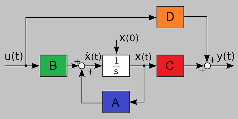
In the modern control theory a system can be represented by the state equation, these are differential equation which can be expressed in a general form as
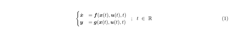
This is an elegant form to represent a system that will be studied and controlled. Here the first equation represents the states' evolution in time, which are the variables that describe the system. The second equation corresponds to the outputs which are those variables that we can measure in reality.
But these equations can be simplified if we regard several facts about certain types of systems we could analyze. If we have a system whose dynamics are independent of the time, and also is linear, the equations turn in
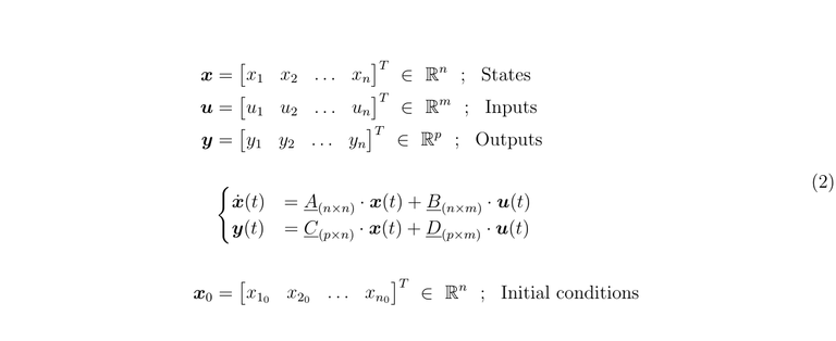
If you are a Control Systems Engineer it is important to know how to resolve this system equation to understand the mechanics involves in your system, and then, be able to control it. To do that, first, let's take a look at an important tool.
The exponential matrix
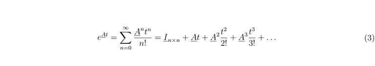
There is an important function that takes place in this resolution, which is the exponential matrix. We can define it as
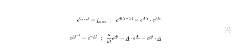
Also, this matrix has to meet the following properties
Solution in the time domain
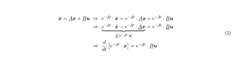
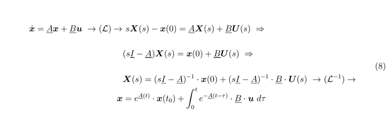
Now we can resolve the state equation in the time domain making use of the exponential matrix and its properties
Let's split the differentials and integrate on the interval that we wish
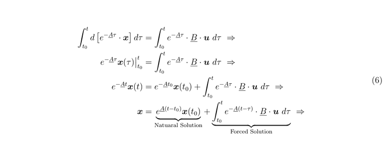
Finally, we can pose the total solution
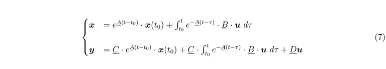
Analyzing this result is not difficult to see that the solution is composed for two sorts of expressions, the first is the natural solution when the output corresponds only to the energy stored in the systems before the input takes place, this energy is stored in the initial conditions. The second sort of solution is that corresponds to the energy that gets into the systems due to the input.
Solution in the frequency domain
It is possible to use the properties of the Laplace Transform to get the solution. But in this way, we can obtain another tool that is important for the systems control and analysis, The Transfer Matrix Function. When it is used The Laplace Environment for this kind of study the norm is to take the initial conditions as zero, but here we are going to consider them differents to cero to make a comparison with the late solution.
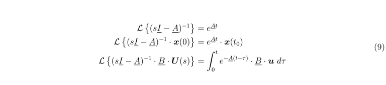
If we compare these results we have
Let's pass to the output equation
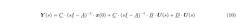
To avoid Dirac deltas in the solution, when we work with the Laplace Transform the initial conditions and the transfer matrix are zero, then, we get
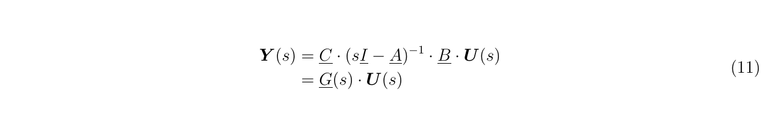
In the past equations, the relation between the input and the output is called The Transfer Function Matrix.
Implementation using difference equation
If we are working with arrays in a computer we can solve the equations in the state space if we make use of equations in differences with a sample time, in this case, we have to compute only two new matrices, let's see
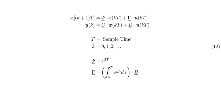
With these equations usual to work in engineering programs to solve the state equations.
MATLAB code
clear all
close all
clc

%%
syms t tau a real
syms s imag

%% The system data

tini = 0;
tfin = 30;
T    = 1e-2;
time = [ tini : T : tfin ];

% u_t =  [ ones(1,length(time)) ;
%         0.5*ones(1,length(time)) ;
%         2*ones(1,length(time)) ];

u_t = ones( 1 , length(time) );

A = [ -8 1 0 ;
      -5 0 1 ;
      -6 0 0 ];

B = [0 ; 1 ; 0];

C = [ 1 0 0 ;
      1 0 1 ;
      1 1 1 ];

D = zeros( length(C(:,1)) , length(B(1,:)) );

x0 = [ 0 ; 1 ; 0 ];

%%

[P1,P2] = eig(A); % Matrix diagonalinzante , diagonal matrix

Phi = round(P1*diag(exp(diag(P2*T)))*inv(P1) , 4);
Gam = round(eval(int(P1*diag(exp(diag(P2*a)))*inv(P1)*B, a , tini, T)),4);

x_k = x0;
x = [ x0 , zeros( 3 , length(time)-2 ) ];
y = zeros( length(C(:,1)) , length(time) );

%%

for k = 1 : length(time)

    if k < length(time)
       x(:,k+1) = Phi*x_k + Gam*u_t(:,k+1);

       x_k = x(:,k+1);
    end
    y(:,k) = C*x_k;

end

%%
figure
subplot(1,2,1)
plot(time,x ,'LineWidth',1.5)
xlabel('time [s]')
ylabel('States')
grid

subplot(1,2,2)
plot( time,y , 'LineWidth',1.5 )
xlabel('time [s]')
ylabel('Outputs')
grid
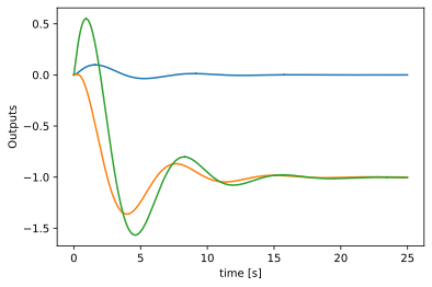
Python Code
try:
    from IPython import get_ipython

    get_ipython().magic('clear')
    get_ipython().magic('reset -f')
    # get_ipython().magic('matplotlib qt')      # plots out line
    get_ipython().magic('matplotlib', 'inline') # plots in line

except:
    pass

import numpy as np
from numpy import *

import control as co

import sympy as smp
from sympy import *

import scipy as scp
from scipy.optimize import *
from scipy.integrate import *

import pandas            as pd
import matplotlib.pyplot as plt
import sklearn           as sk
import math
import os
import tarfile
import urllib

np.set_printoptions(precision=4, suppress=True)
init_printing(use_unicode=True)

#%%

t  =  symbols( 't ' )

tini = 0
tfin = 25
T    = 1e-2

time = np.array( np.arange( tini , tfin , T ) , ndmin=2 )

#%%

A = np.array([[-8, 1, 0, ],
              [-5, 0, 1, ],
              [-6, 0, 0, ]])

B = np.array([[0],
              [1],
              [0]])

C = np.array([[1, 0, 0],
              [1, 0, 1],
              [1, 1, 1]])

D = np.zeros( (len(C[:,1]) , len(B[1,:])) );

x0 = np.array([[0],
               [0],
               [0]] , ndmin = 2 )

u_t = np.ones( (1 , len(time[0,:])) );

#%%

V , R = np.linalg.eig(A) # Eigvalues in a vector, Matrix Diagonalizante

M = np.round( np.linalg.inv(R) @ A @ R , 4) # Diagonal Matrix

ExpA_T = np.diag( e**(V*T) )
ExpA_t = np.diag( e**(V*t) )

Phi = np.round( R @ ExpA_T @ np.linalg.inv(R)   , 4)

inte = smp.Matrix( ( ( R @ ExpA_t @ np.linalg.inv(R) ) @ B ) )

Gam = integrate( expand(inte) , (t , tini , T) )
Gam = np.array( Gam.evalf() , dtype = complex )

#%%

x_k = np.array( x0 , ndmin=2);

z0 = np.zeros( (3 , len(time[0,:])-1 ) )

x = np.hstack( (x0 , z0)  )

y = np.zeros( ( len(C[:,1]) , len(time[0,:]) ) );

#%%


for k in range(len(time[0,:])-1):

    # print(x_k)

    M1 = (Phi @  x_k ).reshape( len(A[0,:]) , 1 )
    M2 = (Gam @  u_t[:,k+1].reshape( len(B[0,:]), 1)).reshape( len(A[0,:]), 1)

    x[:,k+1] = (M1 + M2).reshape( 3 )

    x_k = x[:,k+1]


y1 = C @ x

#%% Plot figure

plt.figure()
plt.plot( time.T  , y1.T )
plt.xlabel('time [s]')
plt.ylabel('Outputs')
plt.plot()