Mathematics - Signals and Systems - LTI System Analysis using Laplace Transform
[Image1]
Introduction
Hey it's a me again @drifter1!
Today we continue with my mathematics series about Signals and Systems in order to cover the LTI System Analysis using Laplace Transform.
So, without further ado, let's get straight into it!
LTI System Properties and Laplace Transform
One very important application of the Laplace Transform is its use in LTI system analysis and classification.
Similar to the more specific Fourier Transform, the usefulness of the Laplace Transform is again a direct result of its convolution property.
Due to this property, the Laplace Transform of the input and output of a given system are related by multiplication with the so called system (or transfer) function H(s), which is the Laplace Transform of the system impulse response.
Mathematically:
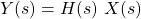
 : Laplace Transform of the system input
 : Laplace Transform of the system output
 : Laplace Transform of the system impulse response
In the case of the Laplace Transform, the system function or block diagram of a given system is not sufficient for the sake of representation. The Region of Convergence (short ROC) is also important to define. More specifically, if the ROC includes the imaginary-axis, then for s = jω the system function H(s) is basically the frequency response of the system. Many such properties can be analyzed in correlation to the system function in the s-plane. Let's get into some of them...
Causality
A system is causal (or satisfies causality) when its response (output) only depends on past and present input, but not future input. In other words, any causal LTI system has a zero impulse response for t < 0. This also means that the system is right-sided. Based on what we covered in the article about the Laplace Transform, this leads us to the conclusion that:
The ROC of the system function of a causal system is a right sub-plane.Of course, the opposite is not always true! A ROC to-the-right of the right-most pole doesn't guarantee that the system is causal, but only that the impulse response is right-sided. But, a rational system function H(s) can be used for concluding that a system is causal, if the ROC is proven to be a right sub-plane, as stated below:
A system with a rational system function is causal, in the case where the ROC is a right sub-plane
to-the-right of the right-most pole.
Its also possible to define the concept of anti-causality, where similar properties are defined for left-sided sub-planes. As such, if the ROC of the system function is a left sub-plane the system is considered anti-causal, which means that H(s) is zero for t > 0. And if the system function is rational, then the system can be considered anti-causal if the ROC is to-the-left of the left-most pole.
Stability
A system is considered stable if bounded input leads to bounded output. This basically means that finite amplitude leads to finite amplitude, or that the system impulse response is absolutely integratable. Because, the Laplace Transform along the jω-axis is equal to the Fourier Transform, it's possible to define stability as:
An LTI system is stable only if the ROC of the system function H(s) includes the jω-axis (i.e. Re{s} = 0)
Stability can be related to causality. But, because its plausible for non-rational system functions to be absolutely integratable, meaning that the system is considered stable, its only possible to relate causality and stability for rational system functions. For a number of systems, its possible to use the position of the poles in order to specify if the system is stable. As such, an causal LTI system with a rational system function, and so with an ROC to-the-right of the right-most pole, is also considered to be stable only if the right-most pole is to-the-left of the jω-axis, or:
A causal system with a rational system function H(s) is stable only if the poles are
in the left-half of the s-plane (i.e. all poles have negative real parts).
LCCDE Representation and Laplace Transform
The properties of the Laplace transform make it very useful in analyzing LTI systems which can be represented using linear constant-coefficient differential equations (short LCCDE). Applying the Laplace Transform to such an differential equation converts the given system to an algebraic expression that relates the Laplace transform of the system output to the product of the Laplace transform of the system input and the sytem function. The system response is afterwards taken using the inverse Laplace Transform.
An LCCDE can be represented as follows:
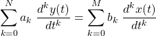
After taking the Laplace Transform of both sides and using linearity and differentation properties, its posible to come up with:
or
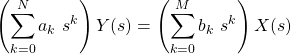
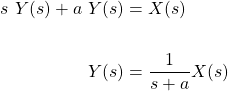
In the article about the Laplace Transform we mentioned that the system function can be represented as the quotient of the zeros and poles:
The two sums of the previous equation can be thought of as exactly that. As such, the roots of the numerator are the zeros of the system function, whilst the roots of the denominator are the poles.
Of course the LCCDE doesn't specify any ROC, but if something like the stability or causality of a given system is known, then its easy to specify the exact ROC!
First-Order System Analysis
First- and second-order systems are quite commonly used as build blocks for larger systems. So, let's get into how the Laplace Transform can be used to describe the behaviour of such systems.
A first-order system can be represented by the following LCCDE:
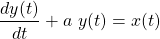
which turns into the following representation after the Laplace Transform is applied:
The system function H(s) is one of the transform table cases, and so its easy to conclude that h(t) can be either of the following:
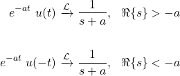
In other words, a first-order system can be represented by a single pole in the s-plane, and have an ROC that is either to-the-right or to-the-left of that pole, depending on other factors such as causality and stability.
Second-Order System Analysis
A second-order system can be represented by an LCCDE of the form:
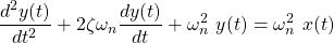
Taking the Laplace Transform results in the following equation:
where the roots of the denominator are as follows:
For ζ < 1:

For such systems, the poles may be in either the real-axis of the s-plane or off the real-axis as a complex conjugate pair (i.e. when ζ < 1), depending on the relation between the coefficients. When both poles are real-valued, the system is referred to as overdamped when ζ > 1 and underdamped when 0 < ζ < 1. As the poles move closer to the jω-axis the damping decreases, whilst when the poles move parallel to the jω-axis the oscillation changes in frequency.
RESOURCES:
References
Images
Mathematical equations used in this article were made using quicklatex.
Block diagrams and other visualizations were made using draw.io and GeoGebra
Previous articles of the series
Basics
- Introduction → Signals, Systems
- Signal Basics → Signal Categorization, Basic Signal Types
- Signal Operations with Examples → Amplitude and Time Operations, Examples
- System Classification with Examples → System Classifications and Properties, Examples
- Sinusoidal and Complex Exponential Signals → Sinusoidal and Exponential Signals in Continuous and Discrete Time
LTI Systems and Convolution
- LTI System Response and Convolution → Linear System Interconnection (Cascade, Parallel, Feedback), Delayed Impulses, Convolution Sum and Integral
- LTI Convolution Properties → Commutative, Associative and Distributive Properties of LTI Convolution
- System Representation in Discrete-Time using Difference Equations → Linear Constant-Coefficient Difference Equations, Block Diagram Representation (Direct Form I and II)
- System Representation in Continuous-Time using Differential Equations → Linear Constant-Coefficient Differential Equations, Block Diagram Representation (Direct Form I and II)
- Exercises on LTI System Properties → Superposition, Impulse Response and System Classification Examples
- Exercise on Convolution → Discrete-Time Convolution Example with the help of visualizations
- Exercises on System Representation using Difference Equations → Simple Block Diagram to LCCDE Example, Direct Form I, II and LCCDE Example
- Exercises on System Representation using Differential Equations → Equation to Block Diagram Example, Direct Form I to Equation Example
Fourier Series and Transform
- Continuous-Time Periodic Signals & Fourier Series → Input Decomposition, Fourier Series, Analysis and Synthesis
- Continuous-Time Aperiodic Signals & Fourier Transform → Aperiodic Signals, Envelope Representation, Fourier and Inverse Fourier Transforms, Fourier Transform for Periodic Signals
- Continuous-Time Fourier Transform Properties → Linearity, Time-Shifting (Translation), Conjugate Symmetry, Time and Frequency Scaling, Duality, Differentiation and Integration, Parseval's Relation, Convolution and Multiplication Properties
- Discrete-Time Fourier Series & Transform → Getting into Discrete-Time, Fourier Series and Transform, Synthesis and Analysis Equations
- Discrete-Time Fourier Transform Properties → Differences with Continuous-Time, Periodicity, Linearity, Time and Frequency Shifting, Conjugate Summetry, Differencing and Accumulation, Time Reversal and Expansion, Differentation in Frequency, Convolution and Multiplication, Dualities
- Exercises on Continuous-Time Fourier Series → Fourier Series Coefficients Calculation from Signal Equation, Signal Graph
- Exercises on Continuous-Time Fourier Transform → Fourier Transform from Signal Graph and Equation, Output of LTI System
- Exercises on Discrete-Time Fourier Series and Transform → Fourier Series Coefficient, Fourier Transform Calculation and LTI System Output
Filtering, Sampling, Modulation, Interpolation
- Filtering → Convolution Property, Ideal Filters, Series R-C Circuit and Moving Average Filter Approximations
- Continuous-Time Modulation → Getting into Modulation, AM and FM, Demodulation
- Discrete-Time Modulation → Applications, Carriers, Modulation/Demodulation, Time-Division Multiplexing
- Sampling → Sampling Theorem, Sampling, Reconstruction and Aliasing
- Interpolation → Reconstruction Procedure, Interpolation (Band-limited, Zero-order hold, First-order hold)
- Processing Continuous-Time Signals as Discrete-Time Signals → C/D and D/C Conversion, Discrete-Time Processing
- Discrete-Time Sampling → Discrete-Time (or Frequency Domain) Sampling, Downsampling / Decimation, Upsampling
- Exercises on Filtering → Filter Properties, Type and Output
- Exercises on Modulation → CT and DT Modulation Examples
- Exercises on Sampling and Interpolation → Graphical/Visual Sampling and Interpolation Examples
Laplace and Z Transforms
- Laplace Transform → Laplace Transform, Region of Convergence (ROC)
- Laplace Transform Properties → Linearity, Time- and Frequency-Shifting, Time-Scaling, Complex Conjugation, Multiplication and Convolution, Differentation in Time- and Frequency-Domain, Integration in Time-Domain, Initial and Final Value Theorems
Final words | Next up
And this is actually it for today's post!
Next time we will get into exercises on the Laplace Transform and LTI System Analysis that is based on it...
See Ya!

Keep on drifting!