Mathematics - Signals and Systems - Continuous-Time to Discrete-Time Design Mapping
[Image1]
Introduction
Hey it's a me again @drifter1!
Today we continue with my mathematics series about Signals and Systems to get into Continuous-Time to Discrete-Time Design Mapping.
So, without further ado, let's dive straight into it!
Small Z-Transform Recap
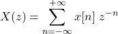
The Z-Transform can be thought of as a generalization of the Discrete-Time Fourier Transform. Using it many systems that normally don't converge (using the Fourier Transform) may be able to converge. Some of the most significant properties of the Transform are linearity, time-shifting and convolution. For example, due to the convolution property, the output of an LTI system can be defined as an product of the Z Transform of the input and the the so called system function H(z) (Z Transform of the system impulse response).
The Z-Transform is also useful when systems are described using linear constant-coefficient difference equations (short LCCDE), as applying the Z-Transform leads to an algebraic expression, which in turn can be solved for the system function. But, the system function alone is not sufficient for representing systems. For any algebraic representation an associated region-of-convergence (ROC) must also be specified. It's easy to derive the ROC from system properties such as causality and stability. Typically, first- or second-order LCCDE's are used as building blocks for higher-order difference equations.
Designing Discrete-Time Systems
When desiging a discrete-time system, one tries to obtain an LCCDE that meets a given set of system specifications. One approach is mapping a continuous-time design to a discrete-time design. This makes a lot of sense, as well-developed continuous-time systems should be used as a reference for a new design. Let's also not forget to mention the concept of sampling, which may closely associates a given discrete-time system with a contiunous-time system.
Sometimes obtaining the difference equation might be as simple as replacing the derivatives in the differential equations that describes the continuous-time system. Using simple forward or backward differences one may obtain an approximate discrete-time difference equation that corresponds to the differential equation. Of course this approach is limited by the mapping from the s-plane to the z-plane, which leads to frequency distortions and sometimes unstable filters.
Another way of mapping the continuous-time system is, by using the so called impulse-invariant design procedure. In this technique, the discrete-time system function is determined by corresponding the impulse response of the discrete-time system to samples of the impulse response of the continuous-time system. This basically leads to a mapping of the poles of the system function, and yields identical (in shape) frequency responses, except for some possible distortion due to aliasing. Thus, this procedure can be safely used with band-limited frequency responses.
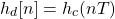
Mapping from Derivatives to Differences
A continuous-time system is represented using differential equations as follows:
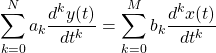
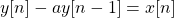
On the other hand, a discrete-time system is represented using difference equations, which lead to:
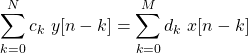
In order to map the top equation to the bottom, two approaches are used:
- Backward Difference
- Forward Difference
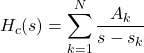
Mapping using Impulse Invariance
When using impulse-invariance the impulse responses of the continuous-time and discrete-time system are related as such:
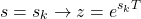
And so, if the Fourier Transform of the continous-time impulse response is of the form:
mapping from one Domain to the other is as simple as:
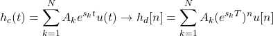
The Z-Transform of the system function is:
It's easy to notice that the coefficients are preserved in all the equations.
Let's also note that the poles can be easily mapped as follows:
First-Order Systems and Z-Transform
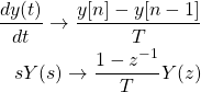
Let's now consider the following basic first-order difference equation:
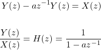
Applying the Z-Transform yields the following system function:
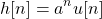
If the system is causal, the ROC is:
and the impulse response is:
Second-Order Systems and Z-Transform
Let's now consider the following second-order difference equation:

The Z-Transform yields the following system function:
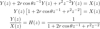
with cosθ < 1 leading to complex poles.
RESOURCES:
References
Images
Mathematical equations used in this article were made using quicklatex.
Block diagrams and other visualizations were made using draw.io
Previous articles of the series
Basics
- Introduction → Signals, Systems
- Signal Basics → Signal Categorization, Basic Signal Types
- Signal Operations with Examples → Amplitude and Time Operations, Examples
- System Classification with Examples → System Classifications and Properties, Examples
- Sinusoidal and Complex Exponential Signals → Sinusoidal and Exponential Signals in Continuous and Discrete Time
LTI Systems and Convolution
- LTI System Response and Convolution → Linear System Interconnection (Cascade, Parallel, Feedback), Delayed Impulses, Convolution Sum and Integral
- LTI Convolution Properties → Commutative, Associative and Distributive Properties of LTI Convolution
- System Representation in Discrete-Time using Difference Equations → Linear Constant-Coefficient Difference Equations, Block Diagram Representation (Direct Form I and II)
- System Representation in Continuous-Time using Differential Equations → Linear Constant-Coefficient Differential Equations, Block Diagram Representation (Direct Form I and II)
- Exercises on LTI System Properties → Superposition, Impulse Response and System Classification Examples
- Exercise on Convolution → Discrete-Time Convolution Example with the help of visualizations
- Exercises on System Representation using Difference Equations → Simple Block Diagram to LCCDE Example, Direct Form I, II and LCCDE Example
- Exercises on System Representation using Differential Equations → Equation to Block Diagram Example, Direct Form I to Equation Example
Fourier Series and Transform
- Continuous-Time Periodic Signals & Fourier Series → Input Decomposition, Fourier Series, Analysis and Synthesis
- Continuous-Time Aperiodic Signals & Fourier Transform → Aperiodic Signals, Envelope Representation, Fourier and Inverse Fourier Transforms, Fourier Transform for Periodic Signals
- Continuous-Time Fourier Transform Properties → Linearity, Time-Shifting (Translation), Conjugate Symmetry, Time and Frequency Scaling, Duality, Differentiation and Integration, Parseval's Relation, Convolution and Multiplication Properties
- Discrete-Time Fourier Series & Transform → Getting into Discrete-Time, Fourier Series and Transform, Synthesis and Analysis Equations
- Discrete-Time Fourier Transform Properties → Differences with Continuous-Time, Periodicity, Linearity, Time and Frequency Shifting, Conjugate Summetry, Differencing and Accumulation, Time Reversal and Expansion, Differentation in Frequency, Convolution and Multiplication, Dualities
- Exercises on Continuous-Time Fourier Series → Fourier Series Coefficients Calculation from Signal Equation, Signal Graph
- Exercises on Continuous-Time Fourier Transform → Fourier Transform from Signal Graph and Equation, Output of LTI System
- Exercises on Discrete-Time Fourier Series and Transform → Fourier Series Coefficient, Fourier Transform Calculation and LTI System Output
Filtering, Sampling, Modulation, Interpolation
- Filtering → Convolution Property, Ideal Filters, Series R-C Circuit and Moving Average Filter Approximations
- Continuous-Time Modulation → Getting into Modulation, AM and FM, Demodulation
- Discrete-Time Modulation → Applications, Carriers, Modulation/Demodulation, Time-Division Multiplexing
- Sampling → Sampling Theorem, Sampling, Reconstruction and Aliasing
- Interpolation → Reconstruction Procedure, Interpolation (Band-limited, Zero-order hold, First-order hold)
- Processing Continuous-Time Signals as Discrete-Time Signals → C/D and D/C Conversion, Discrete-Time Processing
- Discrete-Time Sampling → Discrete-Time (or Frequency Domain) Sampling, Downsampling / Decimation, Upsampling
- Exercises on Filtering → Filter Properties, Type and Output
- Exercises on Modulation → CT and DT Modulation Examples
- Exercises on Sampling and Interpolation → Graphical/Visual Sampling and Interpolation Examples
Laplace and Z Transforms
- Laplace Transform → Laplace Transform, Region of Convergence (ROC)
- Laplace Transform Properties → Linearity, Time- and Frequency-Shifting, Time-Scaling, Complex Conjugation, Multiplication and Convolution, Differentation in Time- and Frequency-Domain, Integration in Time-Domain, Initial and Final Value Theorems
- LTI System Analysis using Laplace Transform → System Properties (Causality, Stability) and ROC, LCCDE Representation and Laplace Transform, First-Order and Second-Order System Analysis
- Exercises on the Laplace Transform → Laplace Transform and ROC Examples, LTI System Analysis Example
- Z Transform → Z Transform, Region of Convergence (ROC), Inverse Z Transform
- Z Transform Properties → Linearity, Time-Shifting, Time-Scaling, Time-Reversal, z-Domain Scaling, Conjugation, Convolution, Differentation in the z-Domain, Initial and Final value Theorems
- LTI System Analysis using Z Transform → System Properties (Causality, Stability), LCCDE Representation and Z Transform
- Exercises on the Z Transform → Z Transform and ROC Examples, ROC from Conditions, LTI System Analysis Example
Final words | Next up
And this is actually it for today's post!
Next up are Butterworth Filters...
See Ya!

Keep on drifting!