Mathematics - Signals and Systems - Butterworth Filters
[Image1]
Introduction
Hey it's a me again @drifter1!
Today we continue with my mathematics series about Signals and Systems to get into Butterworth Filters.
So, without further ado, let's dive straight into it!
Introduction to Butterworth Filters
Butterworth filters apply topics that we discussed in the previous article, which was about discrete-time system design. This useful class of filters is specified by two main parameters:
- Cut-off Frequency (ωc)
- Filter Order (N)

[Image 2]
Applying techniques such as impulse invariance, it's possible to create discrete-time Butterworth filters. The filter specifications can be mapped to a corresponding set of specifications for the discrete-time filter, but there are of course some limitations. In order to avoid aliasing, the continuous-time filter needs to be band-limited. This can be done using a procedure known as bilinear transformation, where the entire imaginary axis in the s-plane is mapped around the unit circle. Since the imaginary axis is of infinite length, a non-linear distortion mapping between the two frequency axes occurs. Thus, even this technique can only be used when the filter is (at least) approximately a constant piecewise function (defined by cases).
Butterworth Filter Equation and Pole-Zero Plot
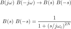
Mathematically, Butterworth filters are defined as:
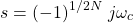
In the s-plane, the square of the magnitude of the frequency response gives us:
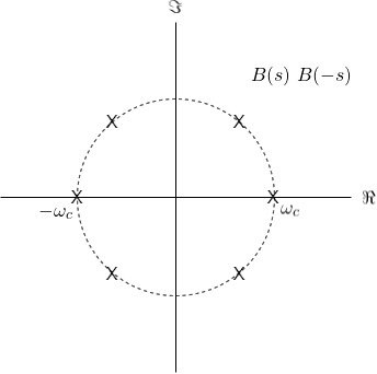
The poles of B(s) B(-s) are at:
which gives us pole-zero patterns of the following form:
Mapping using Impulse Invariance
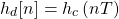
Let's first talk about mapping the filter using Impulse Invariance. The sampled signal is taken as follows:
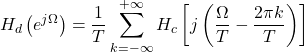
As a Fourier series, the frequency response is defined as:
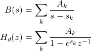
For the Z-Transform, we need to determine B(s) and using partial fraction expansion we come up with:
Mapping using Bilinear Transformation
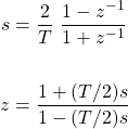
Using Bilinear Transformation, the following mapping occurs:
where s and z are given by:
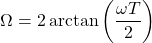
For z = e jΩ, s is given by:
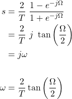
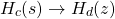
Mapping from the continuous-time frequency axis (ω) to the discrete time frequency axis (Ω) is exactly what the Bilinear Transform is all about. So, in the end, it's basically the following mapping:
RESOURCES:
References
Images
- https://commons.wikimedia.org/wiki/File:From_Continuous_To_Discrete_Fourier_Transform.gif
- https://commons.wikimedia.org/wiki/File:Butterworth_orders.png
Mathematical equations used in this article were made using quicklatex.
Block diagrams and other visualizations were made using draw.io
Previous articles of the series
Basics
- Introduction → Signals, Systems
- Signal Basics → Signal Categorization, Basic Signal Types
- Signal Operations with Examples → Amplitude and Time Operations, Examples
- System Classification with Examples → System Classifications and Properties, Examples
- Sinusoidal and Complex Exponential Signals → Sinusoidal and Exponential Signals in Continuous and Discrete Time
LTI Systems and Convolution
- LTI System Response and Convolution → Linear System Interconnection (Cascade, Parallel, Feedback), Delayed Impulses, Convolution Sum and Integral
- LTI Convolution Properties → Commutative, Associative and Distributive Properties of LTI Convolution
- System Representation in Discrete-Time using Difference Equations → Linear Constant-Coefficient Difference Equations, Block Diagram Representation (Direct Form I and II)
- System Representation in Continuous-Time using Differential Equations → Linear Constant-Coefficient Differential Equations, Block Diagram Representation (Direct Form I and II)
- Exercises on LTI System Properties → Superposition, Impulse Response and System Classification Examples
- Exercise on Convolution → Discrete-Time Convolution Example with the help of visualizations
- Exercises on System Representation using Difference Equations → Simple Block Diagram to LCCDE Example, Direct Form I, II and LCCDE Example
- Exercises on System Representation using Differential Equations → Equation to Block Diagram Example, Direct Form I to Equation Example
Fourier Series and Transform
- Continuous-Time Periodic Signals & Fourier Series → Input Decomposition, Fourier Series, Analysis and Synthesis
- Continuous-Time Aperiodic Signals & Fourier Transform → Aperiodic Signals, Envelope Representation, Fourier and Inverse Fourier Transforms, Fourier Transform for Periodic Signals
- Continuous-Time Fourier Transform Properties → Linearity, Time-Shifting (Translation), Conjugate Symmetry, Time and Frequency Scaling, Duality, Differentiation and Integration, Parseval's Relation, Convolution and Multiplication Properties
- Discrete-Time Fourier Series & Transform → Getting into Discrete-Time, Fourier Series and Transform, Synthesis and Analysis Equations
- Discrete-Time Fourier Transform Properties → Differences with Continuous-Time, Periodicity, Linearity, Time and Frequency Shifting, Conjugate Summetry, Differencing and Accumulation, Time Reversal and Expansion, Differentation in Frequency, Convolution and Multiplication, Dualities
- Exercises on Continuous-Time Fourier Series → Fourier Series Coefficients Calculation from Signal Equation, Signal Graph
- Exercises on Continuous-Time Fourier Transform → Fourier Transform from Signal Graph and Equation, Output of LTI System
- Exercises on Discrete-Time Fourier Series and Transform → Fourier Series Coefficient, Fourier Transform Calculation and LTI System Output
Filtering, Sampling, Modulation, Interpolation
- Filtering → Convolution Property, Ideal Filters, Series R-C Circuit and Moving Average Filter Approximations
- Continuous-Time Modulation → Getting into Modulation, AM and FM, Demodulation
- Discrete-Time Modulation → Applications, Carriers, Modulation/Demodulation, Time-Division Multiplexing
- Sampling → Sampling Theorem, Sampling, Reconstruction and Aliasing
- Interpolation → Reconstruction Procedure, Interpolation (Band-limited, Zero-order hold, First-order hold)
- Processing Continuous-Time Signals as Discrete-Time Signals → C/D and D/C Conversion, Discrete-Time Processing
- Discrete-Time Sampling → Discrete-Time (or Frequency Domain) Sampling, Downsampling / Decimation, Upsampling
- Exercises on Filtering → Filter Properties, Type and Output
- Exercises on Modulation → CT and DT Modulation Examples
- Exercises on Sampling and Interpolation → Graphical/Visual Sampling and Interpolation Examples
Laplace and Z Transforms
- Laplace Transform → Laplace Transform, Region of Convergence (ROC)
- Laplace Transform Properties → Linearity, Time- and Frequency-Shifting, Time-Scaling, Complex Conjugation, Multiplication and Convolution, Differentation in Time- and Frequency-Domain, Integration in Time-Domain, Initial and Final Value Theorems
- LTI System Analysis using Laplace Transform → System Properties (Causality, Stability) and ROC, LCCDE Representation and Laplace Transform, First-Order and Second-Order System Analysis
- Exercises on the Laplace Transform → Laplace Transform and ROC Examples, LTI System Analysis Example
- Z Transform → Z Transform, Region of Convergence (ROC), Inverse Z Transform
- Z Transform Properties → Linearity, Time-Shifting, Time-Scaling, Time-Reversal, z-Domain Scaling, Conjugation, Convolution, Differentation in the z-Domain, Initial and Final value Theorems
- LTI System Analysis using Z Transform → System Properties (Causality, Stability), LCCDE Representation and Z Transform
- Exercises on the Z Transform → Z Transform and ROC Examples, ROC from Conditions, LTI System Analysis Example
- Continuous-Time to Discrete-Time Design Mapping → Discrete-Time System Design Techniques (Mapping from Derivatives to Differences, Mapping using Impulse Invariance), First- and Second-Order Systems and Z-Transform
Final words | Next up
And this is actually it for today's post!
Next up is System Feedback...
See Ya!

Keep on drifting!