Determining Macro Cell Coverage Based on Okumura Hata in Matlab
Note
This is English translated of my undergraduate assignment in Wireless Network course at the Department of Electrical Engineering, Faculty of Engineering, Udayana University. This assignment has never been published anywhere and I, as the author and copyright holder, license this assignment as customized CC-BY-SA where anyone can share, copy, republish, and sell on condition to state my name as the author and notify that the original and open version available here.
Chapter 1 Introduction
1.1 Background
The signal strength received on the MS (Mobile Station) from the BS (Base Station) is generally affected at 3 stages. The first stage is signal generation at the BS (Base Station), the second stage is propagation, and the third stage is the MS (Mobile Station). Until now, there has not been an empirical calculation of signal propagation, which is currently used is prediction based on experiment and research (no theory). One of them is Okumura-Hata where researchers from Japan surround urban, suburban, and rural areas, trying certain distances and measuring the signal obtained by MS (Mobile Station) from BS (Base Station). To measure signal strength using Okumura must provide many tables based on the situation of the area. Even though using Okumura is accurate, it wastes time because we have to check the tables. Hata derived the calculation formula from Okumura but it also took a long time to compute manually. In this paper, calculations will be made from BS (Base Station) to MS (Mobile Station) based on the Hata formula in MATLAB software based on some data. What is calculated is the RX (Received) Power at MS (Mobile Station) in Urban, Suburban, and Rural areas from a distance of 1 km to 20 km.
1.2 Problem
What are the results of the calculation of receiver power in MS (Mobile Station) from transmitter BS (Base Station) in urban, suburban, and rural areas based on the Hata formula using MATLAB software?
1.3 Objective
To make signal propagation calculations from BS (Base Station) to MS (Mobile Station) based on Okumura-Hata in MATLAB.
1.4 Benefit
It is more energy and time efficient to find signal propagation calculations.
1.5 Scope and Limits
- Calculation at a distance of 1 - 20 Km.
- Signal at 900 MHz.
- The tool specifications have been determined.
Chapter 2 Literature Review
2.1 Signal Strength
The unit of signal strength is the watt, which is the unit of power in electricity. To facilitate the calculation of the signal strength from watts it is converted into decibell units (Kolawole, 2002).
Where:
P = Electrical power (watt)2.2 Free Space Loss
Free Space Loss is the signal strength loss in a vacuum, depending on wavelength and distance. This is a loss that must exist (Kolawole, 2002).
Where:
FSL = Free Space Loss
r = the distance between the transmitter and the receiver (meter)
lamda = wavelength (meter)
c = speed of light (meter/second)
2.3 Hata Path Loss
Until now, the empirical formula for calculating the signal strength from BS (Base Station) to MS (Mobile Station) has not been found in the real world environment. What does exist is an approximate prediction based on research. Okumura and Hata surround an area at certain intensities and record the signal strength received by the MS (Mobile Station) from the BS (Base Station) at certain distances. The calculation of the Hata model is as follows (ETSI, 1999):
Limitation:
Frequency (f): 150 - 1000 MHz
Base Station Height (Hb): 30 - 200 m
Mobile Height (Hm): 1 - 10 m
Distance (d): 1 - 20 km
Untuk wilayah metropolitan:
a(Hm)= f ≤ 200 MHz
a(Hm)= f ≥ 400 MHz
For nonmetropolitan areas:
a(Hm)=
Loss for Urban area: 6.55log(Hb)log(d)
Loss for Suburban area
Loss for Rural Quasi-Open area
Loss for Rural Open-Area
2.4 Link Budget
In general, there are 3 steps to calculate the signal strength from the BS (Base Station) to the MS (Mobile Station). The first stage is the signal strength generated by the BS (Base Station) affected by the smear loss and gain that occurs at the BS (Base Station). The second stage is the path loss, it can be calculated with Hata. The third stage is the gain and loss that occurs in MS (Mobile Station). Therefore it can be calculated (ETSI, 1999):
Where:
Pm = Signal strength on MS
Pb = Signal strength on BS
Gb = Gain Atenna BS
Ld = Duplexer Loss BS
Lj = Jumper Loss BS
Lf = Feeder Loss BS
Ltf = Filter Loss BS
Mf = Fade Margin
Ab = Body Atennuation
Av = Vehide Atennuation
Abd = Building Atennuation
Lpj = Path loss
Lm = Feeder Loss MS
Gm = Gain Atenna MS
Lo = Other Loss
2.5 MATLAB
MATLAB is a high-level language and an interactive environment for numerical computation, visualization, and programming. Using MATLAB, you can analyze data, develop algorithms, and create models and applications. Languages, tools, and built-in math functions allow you to explore multiple approaches and reach solutions faster than traditional spreadsheets or programming languages, such as C / C ++ or Java. MATLAB can be used for a wide variety of applications, including signal processing and communications, image and video processing, control systems, test and measurement, computational finance, and computational biology. More than one million engineers and scientists in industry and academia use MATLAB, the language of technical computing (Little, 2013).
Chapter 3 Experimental Method
3.1 Place and Time of Experiment
The experiment was carried out at home on May 22, 2013.
3.2 Tools
3.3 Program
Created 3 programs. The first program to calculate the path loss according to Hata for urban, suburban, and rural areas with distances of 1km, 2km, 3km, 4km, 5km, 6km, 7km, 8km, 9km, 10km, 11km, 12km, 13km, 14km, 15km, 16km, 17km, 18km, 19km, 20km. The second program is product loss, which is the sum of the path loss and indoor propagation loss. The third program for calculating the RX signal strength based on TX, gain, and loss on the device. Can also be made in simulink.
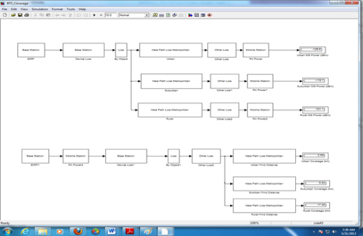
Figure 3.1 In simulink form
%Hata Model%Frequency 150 – 1000 (MHz)
f = 900;

%Base station height 30 – 200 (m)
Hb = 40;

%Mobile Height 1 – 10 (m)
Hm = 1.5;

%Distance 1 – 20 (km)
d = 1:20;

%Urban Area Loss small medium city (dB)
asm = (((1.1*log10(f))-0.7)*Hm)-((1.56*log10(f))-0.8);
Lusm = 69.55 + (26.16*log10(f)) – (13.82*log10(Hb)) – asm + ((44.9 – (6.55*log10(Hb)))*log10(d));

%Urban Area Loss large city (dB)
if f <= 200
    al = (8.29*(log10(1.54*Hm).^2))-1.1;
    Lul = 69.55 + (26.16*log10(f)) – (13.82*log10(Hb)) – al + ((44.9 – (6.55*log10(Hb)))*log10(d));
else if f >= 400
    al = (3.2*(log10(11.75*Hm).^2))-4.97;
    Lul = 69.55 + (26.16*log10(f)) – (13.82*log10(Hb)) – al + ((44.9 – (6.55*log10(Hb)))*log10(d));
else
    ‘frequency range undefine’;
end

%Suburban Area Loss small medium city (dB)
Lsusm = Lusm – (2*(log10(f/28).^2))-5.4;

%Suburban Area large city (dB)
Lsul = Lul – (2*(log10(f/28).^2))-5.4;

%Rural Area small medium city (Quasi-Open) (dB)
Lrqosm = Lusm – (4.78*(log10(f).^2))+(18.33*log10(f))-35.94;

%Rural Area large city (Quasi-Open) (dB)
Lrqol = Lul – (4.78*(log10(f).^2))+(18.33*log10(f))-35.94;

%Rural Area small medium city (Open Area) (dB)
Lrosm = Lusm – (4.78*(log10(f).^2))+(18.33*log10(f))-40.94;

%Rural Area large city (Open Area) (dB)
Lrol = Lul – (4.78*(log10(f).^2))+(18.33*log10(f))-40.94;

subplot(2,1,1);
plot(d,Lusm,d,Lsusm,d,Lrqosm,d,Lrosm);
grid on;
subplot(2,1,2);
plot(d,Lul,d,Lsul,d,Lrqol,d,Lrol);
grid on;
Code 3.1 Path Loss Hata Model
%Product Loss%u = urban %s = surban
%r = rural

%Total Path Loss (dB)
Lptu = Lul;
Lpts = Lsul;
Lptr = Lrol;

%Building Attenuation (dB)
Abdu = 15;
Abds = 12;
Abdr = 0;

%Vhide Attenuation (dB)
Avu = 0;
Avs = 0;
Avr = 0;

%Body Attenuation (dB)
Abu = 2;
Abs = 2;
Abr = 2;

%Fade Margin (dB)
Mfu = 5.6;
Mfs = 5.6;
Mfr = 5.6;

%Feeder loss per meter (dB/m)
Lf_m = 0.0646;

%Feeder loss (dB)
Lf = Hb*Lf_m;

%Product Loss (dB)
Lpu = Lptu + Abdu + Avu + Abu + Mfu + Lf;
Lps = Lpts + Abds + Avs + Abs + Mfs + Lf;
Lpr = Lptr + Abdr + Avr + Abr + Mfr + Lf;
Code 3.2 Product Loss
%MS_BS RX Power%u = urban %s = surban
%r = rural

%MS TX Power (dBm)
Pm = 30;

%MS Antenna Gain (dBi)
Gm = 2;

%MS Feeder Loss (dB)
Lm = 0;

%BS TX Power (dBm)
Pb = 47;

%BS Antenna Gain (dBi)
Gb = 20;

%BS Diversity Gain (dB)
Gd = 3.5;

%BS Duplexer Loss (dB)
Ld = 0.8;

%BS Jumper/Connector Loss (dB)
Lj = 0.9;

%BS TX Filter Loss (dB)
Ltf = 2.3;

%Other Loss (dB)
Lo = 0;

%BS RX Power
Sbu = Pm + Gm – Lm + Gb + Gd – Ld – Lj – Lpu – Lo;
Sbs = Pm + Gm – Lm + Gb + Gd – Ld – Lj – Lps – Lo;
Sbr = Pm + Gm – Lm + Gb + Gd – Ld – Lj – Lpr – Lo;

%MS RX Power
Smu = Gm – Lm + Pb + Gb – Ld – Lj – Ltf – Lpu – Lo;
Sms = Gm – Lm + Pb + Gb – Ld – Lj – Ltf – Lps – Lo;
Smr = Gm – Lm + Pb + Gb – Ld – Lj – Ltf – Lpr – Lo;

plot(d,Smu,d,Sms,d,Smr);
legend(‘Urban’, ‘Suburban’, ‘Rural’);
title(‘Received Power’);
xlabel(‘Distance (km)’);
ylabel(‘Power (dBm)’);
grid on;
Code 3.3 BS MS Power
a = 20; b = 20; ang=0:0.01:2*pi;
x1=d(1)*cos(ang);
y1=d(1)*sin(ang);
x2=d(2)*cos(ang);
y2=d(2)*sin(ang);
x3=d(3)*cos(ang);
y3=d(3)*sin(ang);
x4=d(4)*cos(ang);
y4=d(4)*sin(ang);
x5=d(5)*cos(ang);
y5=d(5)*sin(ang);
x6=d(6)*cos(ang);
y6=d(6)*sin(ang);
x7=d(7)*cos(ang);
y7=d(7)*sin(ang);
x8=d(8)*cos(ang);
y8=d(8)*sin(ang);
x9=d(9)*cos(ang);
y9=d(9)*sin(ang);
x10=d(10)*cos(ang);
y10=d(10)*sin(ang);
x11=d(11)*cos(ang);
y11=d(11)*sin(ang);
x12=d(12)*cos(ang);
y12=d(12)*sin(ang);
x13=d(13)*cos(ang);
y13=d(13)*sin(ang);
x14=d(14)*cos(ang);
y14=d(14)*sin(ang);
x15=d(15)*cos(ang);
y15=d(15)*sin(ang);
x16=d(16)*cos(ang);
y16=d(16)*sin(ang);
x17=d(17)*cos(ang);
y17=d(17)*sin(ang);
x18=d(18)*cos(ang);
y18=d(18)*sin(ang);
x19=d(19)*cos(ang);
y19=d(19)*sin(ang);
x20=d(20)*cos(ang);
y20=d(20)*sin(ang);

%plot(a+x1,b+y1,a+x2,b+y2,a+x3,b+y3,a+x4,b+y4,a+x5,b+y5,a+x6,b+y6,a+x7,b+y7,a+x8,b+y8,a+x9,b+y9,a+x10,b+y10,a+x11,b+y11,a+x12,b+y12,a+x13,b+y13,a+x14,b+y14,a+x15,b+y15,a+x16,b+y16,a+x17,b+y17,a+x18,b+y18,a+x19,b+y19,a+x20,b+y20);
fill(a+x20,b+y20,[0.4 0 0],a+x19,b+y19,[0.6 0 0],a+x18,b+y18,[0.9 0 0],a+x17,b+y17,[1 0.2 0],a+x16,b+y16,[1 0.4 0],a+x15,b+y15,[1 0.7 0],…
a+x14,b+y14,[1 0.9 0],a+x13,b+y13,[0.8 1 0],a+x12,b+y12,[0.6 1 0],a+x11,b+y11,[0 1 0.3],a+x10,b+y10,[0 1 0.5],a+x9,b+y9,[0 1 0.7],…
a+x8,b+y8,[0 1 0.9],a+x7,b+y7,[0 1 1],a+x6,b+y6,[0 0.7 1],a+x5,b+y5,[0 0.6 1],a+x4,b+y4,[0 0.4 1],a+x3,b+y3,[0 0.3 1],…
a+x2,b+y2,[0 0.2 1],a+x1,b+y1,[0 0 1]);
colorbar(‘YTickLabel’,{‘0’,Smu(2),Smu(4),Smu(6),Smu(8),Smu(10),Smu(12),Smu(14),Smu(16),Smu(18),Smu(20)});
grid on;
xlabel(‘X-distance (km)’); %# Add an x axis label
ylabel(‘Y-distance (km)’); %# Add a y axis label
subplot(3,1,1);
Code 3.4 Coverage 1/2
fill(a+x20,b+y20,[0.4 0 0],a+x19,b+y19,[0.6 0 0],a+x18,b+y18,[0.9 0 0],a+x17,b+y17,[1 0.2 0],a+x16,b+y16,[1 0.4 0],a+x15,b+y15,[1 0.7 0],…a+x14,b+y14,[1 0.9 0],a+x13,b+y13,[0.8 1 0],a+x12,b+y12,[0.6 1 0],a+x11,b+y11,[0 1 0.3],a+x10,b+y10,[0 1 0.5],a+x9,b+y9,[0 1 0.7],… a+x8,b+y8,[0 1 0.9],a+x7,b+y7,[0 1 1],a+x6,b+y6,[0 0.7 1],a+x5,b+y5,[0 0.6 1],a+x4,b+y4,[0 0.4 1],a+x3,b+y3,[0 0.3 1],…
a+x2,b+y2,[0 0.2 1],a+x1,b+y1,[0 0 1]);
colorbar(‘YTickLabel’,{‘0’,Smu(4),Smu(8),Smu(15),Smu(17),Smu(20)});
grid on;
xlabel(‘X-distance (km)’); %# Add an x axis label
ylabel(‘Y-distance (km)’); %# Add a y axis label
subplot(3,1,2);

fill(a+x20,b+y20,[0.4 0 0],a+x19,b+y19,[0.6 0 0],a+x18,b+y18,[0.9 0 0],a+x17,b+y17,[1 0.2 0],a+x16,b+y16,[1 0.4 0],a+x15,b+y15,[1 0.7 0],…
a+x14,b+y14,[1 0.9 0],a+x13,b+y13,[0.8 1 0],a+x12,b+y12,[0.6 1 0],a+x11,b+y11,[0 1 0.3],a+x10,b+y10,[0 1 0.5],a+x9,b+y9,[0 1 0.7],…
a+x8,b+y8,[0 1 0.9],a+x7,b+y7,[0 1 1],a+x6,b+y6,[0 0.7 1],a+x5,b+y5,[0 0.6 1],a+x4,b+y4,[0 0.4 1],a+x3,b+y3,[0 0.3 1],…
a+x2,b+y2,[0 0.2 1],a+x1,b+y1,[0 0 1]);
colorbar(‘YTickLabel’,{‘0’,Sms(4),Sms(8),Sms(15),Sms(17),Sms(20)});
grid on;
xlabel(‘X-distance (km)’); %# Add an x axis label
ylabel(‘Y-distance (km)’); %# Add a y axis label
subplot(3,1,3);

fill(a+x20,b+y20,[0.4 0 0],a+x19,b+y19,[0.6 0 0],a+x18,b+y18,[0.9 0 0],a+x17,b+y17,[1 0.2 0],a+x16,b+y16,[1 0.4 0],a+x15,b+y15,[1 0.7 0],…
a+x14,b+y14,[1 0.9 0],a+x13,b+y13,[0.8 1 0],a+x12,b+y12,[0.6 1 0],a+x11,b+y11,[0 1 0.3],a+x10,b+y10,[0 1 0.5],a+x9,b+y9,[0 1 0.7],…
a+x8,b+y8,[0 1 0.9],a+x7,b+y7,[0 1 1],a+x6,b+y6,[0 0.7 1],a+x5,b+y5,[0 0.6 1],a+x4,b+y4,[0 0.4 1],a+x3,b+y3,[0 0.3 1],…
a+x2,b+y2,[0 0.2 1],a+x1,b+y1,[0 0 1]);
colorbar(‘YTickLabel’,{‘0’,Smr(4),Smr(8),Smr(15),Smr(17),Smr(20)});
grid on;
xlabel(‘X-distance (km)’); %# Add an x axis label
ylabel(‘Y-distance (km)’); %# Add a y axis label
Code 3.5 Coverage 2/2
3.4 Input
| NO | Tools | Spesification | Software |
|---|---|---|---|
| 1 | PC | Intel® Pentium® core-i5 processor 4 GB RAM 2 GB VGA Operating System Windows 7 Ultimate 2 | MATLAB 2010 |
| Frequency (f) | 900 MHz |
| Base Station Height (Hb) | 40 m |
| Mobile Station Height (Hm) | 1.5 m |
| Distance (d) | 1:20 km |
| BS Power (dBm) | 47 |
| BS Antenna Gain (dBi) | 20 |
| MS Antenna Gain (dBi) | 2 |
| BS Duplexer Loss (dB) | 0.8 |
| BS Jumper/Connector Loss (dB) | 0.9 |
| BS Filter Loss (dB) | 2.3 |
| Description | Urban | Suburban | Rural |
|---|---|---|---|
| Fade Margin (dB) | 5.6 | 5.6 | 5.6 |
| Feeder Loss / Meter (dB/m) | 0.0646 | 0.0646 | 0.0646 |
| Body Atennuation (dB) | 2 | 2 | 2 |
| Building Atennuation (dB) | 15 | 12 | 0 |
3.5 Output
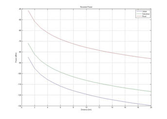
Figure 3.2 Graph of distance to MS power
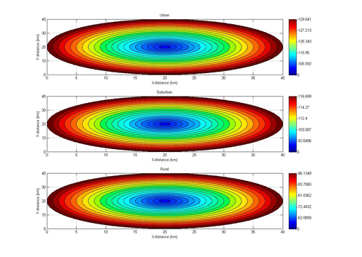
Figure 3.3 MS power at a distance of 1:20 km
Chapter 4 Discussion
4.1 Signal Strength in MS (Mobile Station)
It can be seen in Figure 3.1 that the signal strength decreases exponentially with the distance between the MS (Mobile Station) and the BS (Base Station). According to Hata and Free Space Loss, the signal loss will get bigger as the distance value increases (d). A clearer graphic can be seen in Figure 4.1.
%20diperbesar.png)
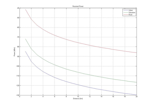
Figure 4.1 Enlarged distance graph to MS (Mobile Station)
From the graph above, it can be seen that the Hata formula shows that urban MS (Mobile Station) has the lowest signal strength value compared to suburban and rural areas. Meanwhile, rural areas have the highest signal strength. If using the Hata formula at a distance of 20 km, the Mobile must have a minimum sensitivity of -130 dBm in urban areas, -117 dBm in suburban areas, and -86 dBm in rural areas. Using MATLAB can also illustrate the value of the MS signal strength in the form of a map at a certain radius as follows with the BS in the middle:
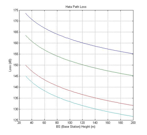
Figure 4.2 MS power at a distance of 1:20 km is enlarged
The graph and image above are the values:
6.55log(Hb))log(d)
With input variations d = 1 km to d = 20 km. The formula above is Loss according to the Hata Model. The formula is based on the ETSI 1999 standard.
4.2 Increase MS Power
4.2.1 Minimizes Hata Path Loss
At first glance the Hata formula does not appear whether the frequency or high parameters of the BTS should be increased or decreased. The distance and height variables MS are natural so they cannot be adjusted. If you use MATLAB, you can see the effect of frequency and height of BTS on loss (with d = 20 km and Hm = 1.5 m).

Figure 4.3 Graph of Path Loss to Base Station Height
From the graph above, it can be seen that the Path Loss will decrease when the BS (Base Station) gets higher. Therefore increasing the BTS height is one solution to reduce loss. The graph above shows the values:
6.55log(Hb))log(d)
With a variation of input Hb = 30 m to d = 200 m. The formula above is Loss according to the Hata Model. The formula is based on the ETSI 1999 standard.
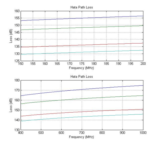
Figure 4.4 Graph of Path Loss to Frequency
From the chart above, it can be seen that the Path Loss will increase the higher the frequency. The graph above shows the values:
6.55log(Hb))log(d)
With input variations f = 150 MHz to f = 1000 MHz. The formula above is Loss according to the Hata Model. The formula is based on the ETSI 1999 standard.
4.2.2 Increasing Tool Specifications
Based on the link budget formula from ETSI 1999:
A higher MS (Mobile Station) signal strength value can be achieved by increasing antenna gain, increasing BS (Base Station) transmit power, and minimizing device loss.
Chapter 5 Closing
5.1 Conclusion
Using MATLAB is much faster than manual counting and can graph and illustrate a BS (Base Station) radius illustration with MS (Mobile Station). From the MATLAB results at a distance of 1 km, the signal strength of MS is -85 dBm in urban areas, -72 dBm in suburban areas, and -8-41 dBm in rural areas. At the farthest distance of 20 km, the signal strength of MS is -130 dBm in urban areas, -117 dBm in suburban areas, and -86 dBm in rural areas.
Bibliography
- ETSI. 1999. ETSI TR 101 362 V8.3.0 (2000-04). Sophia Antipolis Cedex : France.
- Kolawole, M. 2002. Satellite Communication Engineering. Marced Deker, inc : New York
- Little, J. 2013. http://www.mathworks.com/products/matlab. Access 27 Mei 2013.
Mirror
- https://www.publish0x.com/fajar-purnama-academics/determining-macro-cell-coverage-based-on-okumura-hata-in-mat-xolvypz?a=4oeEw0Yb0B&tid=hive
- https://0fajarpurnama0.github.io/bachelor/2020/11/04/determining-macro-cell-coverage-based-on-okumura-hata-in-matlab
- https://0fajarpurnama0.medium.com/determining-macro-cell-coverage-based-on-okumura-hata-in-matlab-f01bfd54fc2b
- https://hicc.cs.kumamoto-u.ac.jp/~fajar/bachelor/determining-macro-cell-coverage-based-on-okumura-hata-in-matlab
- https://0darkking0.blogspot.com/2020/11/determining-macro-cell-coverage-based.html
- https://0fajarpurnama0.cloudaccess.host/index.php/9-fajar-purnama-academics/98-determining-macro-cell-coverage-based-on-okumura-hata-in-matlab
- http://0fajarpurnama0.weebly.com/blog/determining-macro-cell-coverage-based-on-okumura-hata-in-matlab
- https://0fajarpurnama0.wixsite.com/0fajarpurnama0/post/determining-macro-cell-coverage-based-on-okumura-hata-in-matlab
- https://read.cash/@FajarPurnama/determining-macro-cell-coverage-based-on-okumura-hata-in-matlab-1a6bf7fd
- https://www.uptrennd.com/post-detail/determining-macro-cell-coverage-based-on-okumura-hata-in-matlab~ODA3Njg4