I can solve your (Electrical Engineering) exercises!

Let me share with you these seven exercises that were given to me to solve through the internet. The topics involve here are, electrical circuits, control engineering, electrical motors (DC machine en this case), and magnetic circuits. There is a simple math exercise as a bonus related to the Dirac Delta. I hope you can find the resolution nice to read and get general-useful knowledge about Electrical Engineering.
Exercise 0: Mathematics
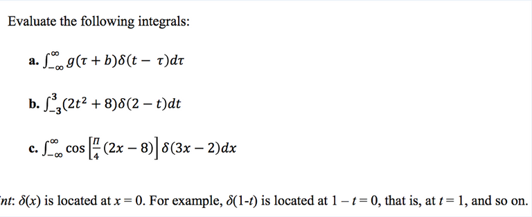
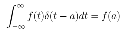
First, we need to know some properties about distributions and the Dirac's Delta δ(t) that we are going to use here
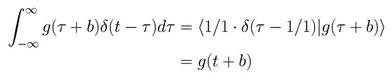
The more important is
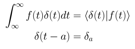
We can use the next short notation
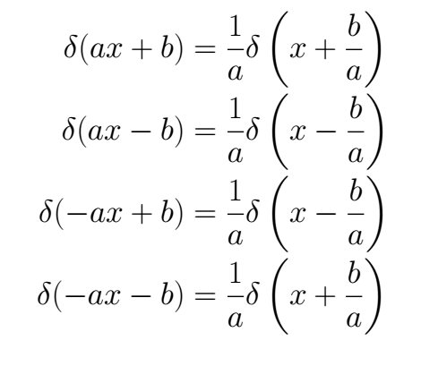
It is possible demostrate that, if a,b > 0
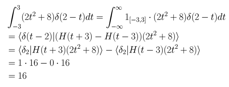
Solving a)
Solving b)
If we think in a function 1_[-3,3] = H(t+3) - H(t-3), where H(t) is the function of Heaviside, then, this function 1_[-3,3] get the value of zero outside the interval [-3,3] and get the value of 1 inside the interval 1_[-3,3].
We can write the integral in this way
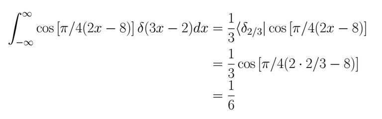
Solving c)
Joining all that we've already learned, this exercise is simple
Exercise 1: Voltage-current- power
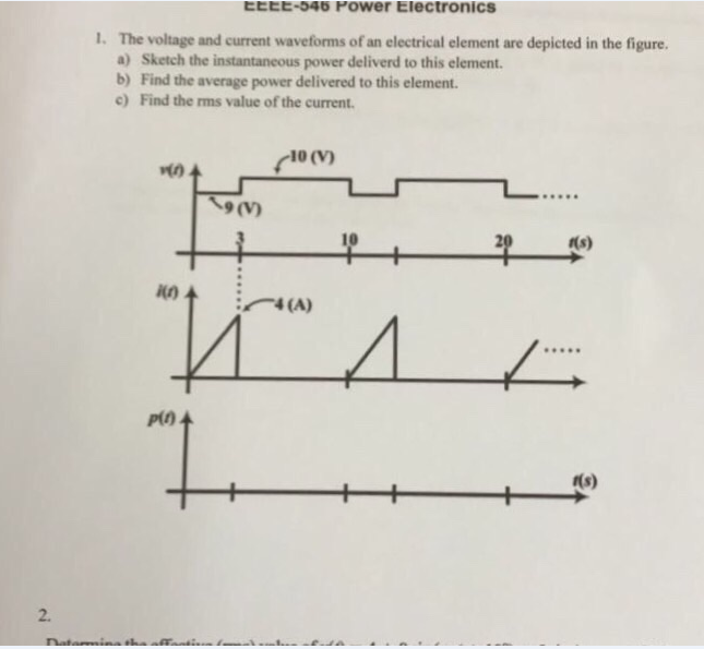
Solving a)
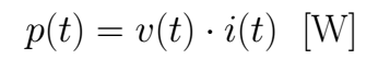
By definition the instantaneous power delivered to an element when voltage and current are known is
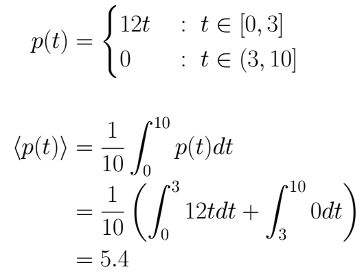
Thus, we have to multiply each point in time between current and voltage, in this case, when the i(t)=0 → p(t) = 10 · 0 = 0 and when i(t) is a line, each point in the line is multiplied by 9 [V], then
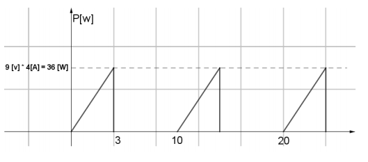
Solving b)
By definition, the mean value of a function f(t) in an interval with amplitude T is
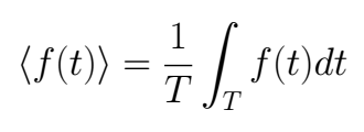
The average power delivered to this device matches with the mean value of the p(t), then
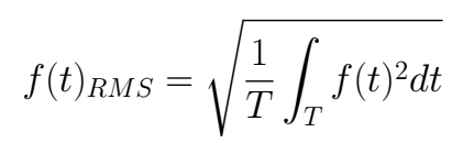
Solving c)
By definition, the Root Mean Square of a function f(t) in an interval with amplitude T is
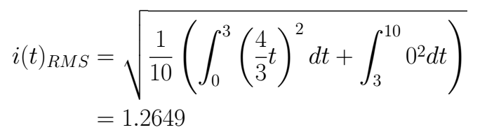
The function which describes the current i(t) is
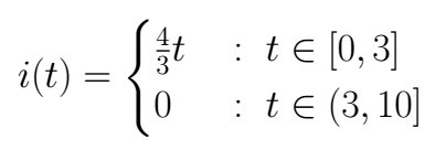
Then
Exercise 2: Electric Circuits
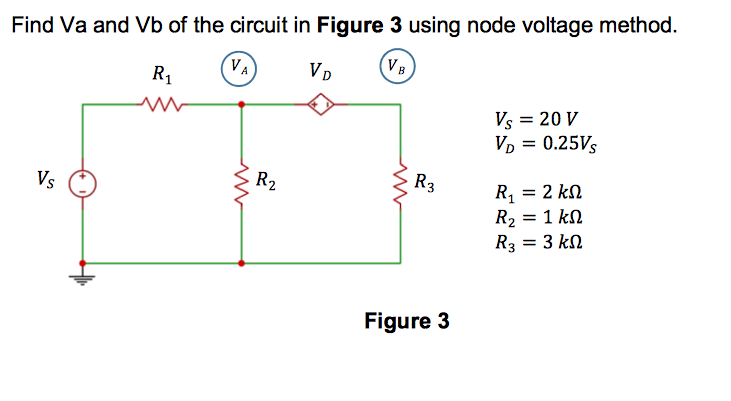
Step 1
Let's assume one path for each current involved, at the beginning this assumption can be wrong for its the direction, but once the calculations are done, the sign (in the current) is going to indicate if our assumption was right.
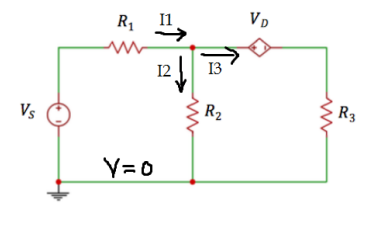
Step 2
Let's pose the equations involved around the node in A, theses are going to be based in the Ohm Law Vi - Vj = RI
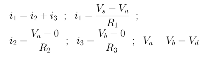
Applying some elementary algebra it is possible to get the following equations
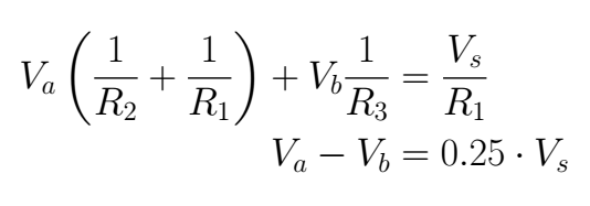
Step 3
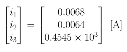
Now is possible to establish the equation system and solve it
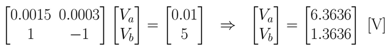
This is the answer, we can see that it meets the condition around the Vd. It is important to verify the resulting currents in order to check up if our assumptions were right, if the signs are +, then we did it well
Exercise 3: Control Engineering (Transfer function)
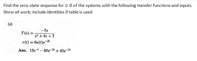
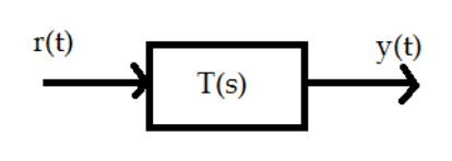
It is always important to represent the system as a block diagram to understand the path of the signals, in this case, only input and output
We are going to resolve this problem using the Laplace Transform, for that, first we transform the input signal. We are going to need the next properties
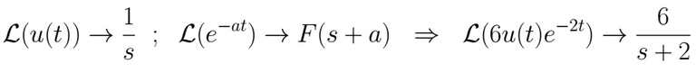
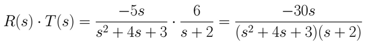
Following the input signal, this is going to be multiplied by the system, which is represented by the Transfer Function $T(s)$, thus, in the frequency domain we get
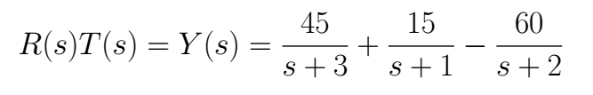
It will be used the partial fractions method to return to the time domain, then, is important to factorize the denominator and to expand the partial fractions in order to find the coefficients in the numerator
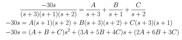
Now, let's pose the equation system matching the factors in the previous expression, it can be solved in the easier way for the student, here, we are going to show the matrix system
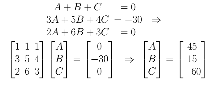
Now, we can write
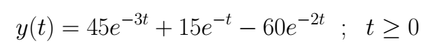
To accomplish the return to the time domain, it is necessary to use the next property
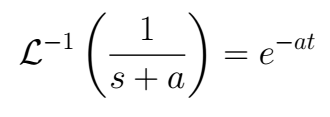
Finally
Exercise 4: Control Engineering (State-space)
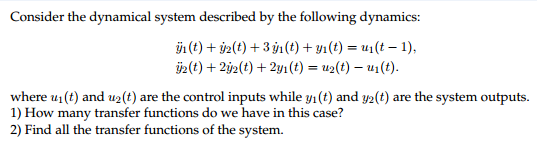
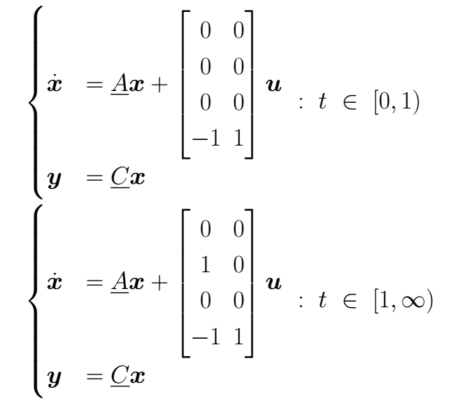
It is possible to answer the two questions finding the transfer function matrix, for this, we are going to take the system towards the state space topology. First, let's declare the state variables regarding until the (n-1) derivative, this is
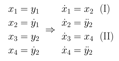
Then, the originals equations change to
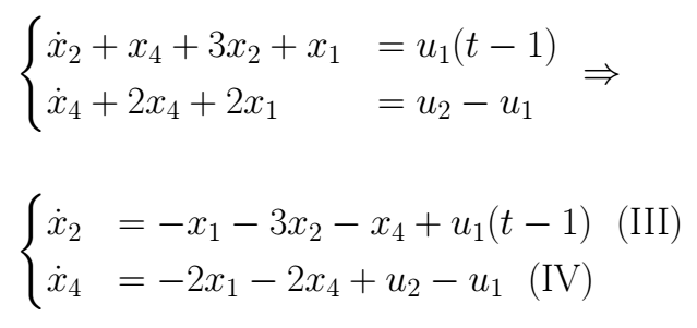
Using (I), (II), (III) y (IV) it is possible to build the state equation of the system in the form
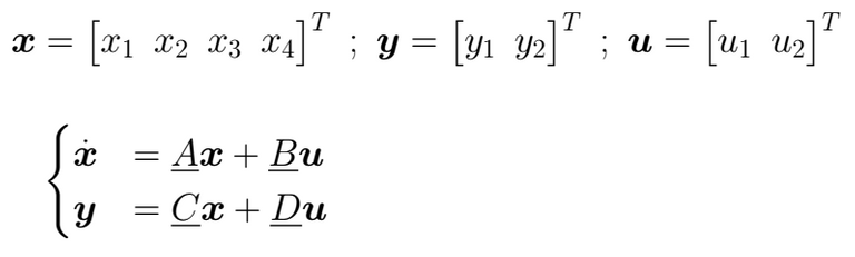
It is not difficult to see that in any case
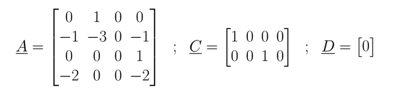
But is important to be careful with the B matrix. When t ∈ [0 , 1] the input u1 in (III) it doesn't take place, only by the time t > 1 it appears in (III). Because of this, we are going to have an equation set for the first time interval, and another equations set for the second time interval; each one of those describes the system behavior in its own time interval.
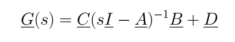
To compute the transfer function matrix G(s) we need to know that
We can handle the issue with the input matrix easily remember that
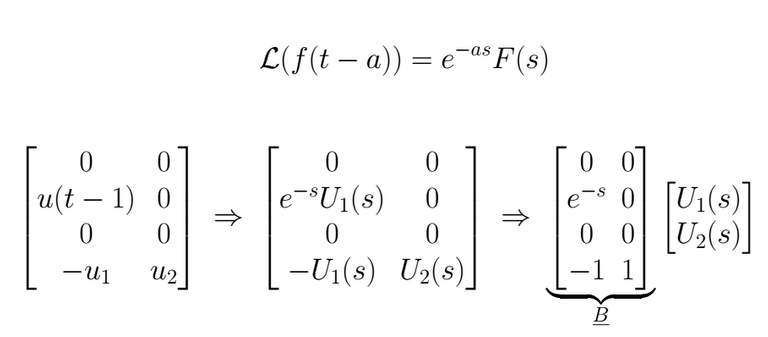
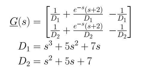
Making the operations, we have
Exercise 5: Control Engineering (Block Diagram - 2 order system)
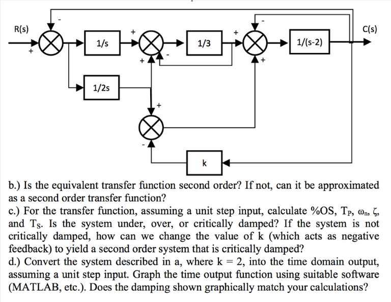
Our first step has to be the reduction of the block diagram using the interaction between the signals inside it. For that, we are going to proceed as follows.
It is always recommended to show all the sum-symbols with only two signals in its inputs, for that, we created a new sum-symbol (N2) next to the first that we've just split in two signals input (N1), in this new sum-symbol we add the last signal and the result of the symbol N1. Then, if some simple reductions have appeared we solve them. These steps are that we've done in the first reduction showed on the next page figure.
Once the diagram looks simpler we identify the signals' ''name'' in order to understand which are the operations that take place over them. Finally, we can follow the signals and build the equations which represent the dynamic inside the diagram. Is useful to label the signals in the output of the sum-symbols. When this has been done, we can build the equations which represent the operations over such signals and finally solve for the system output, in this case, C(s). These have been the finals steps in the next page figure.
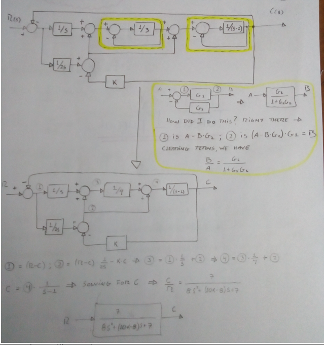
As we can see this system is the second-order and can be handled with the elemental equations used for its kind. All the results will be dependents of K. The next figure shows the equations and calculations.
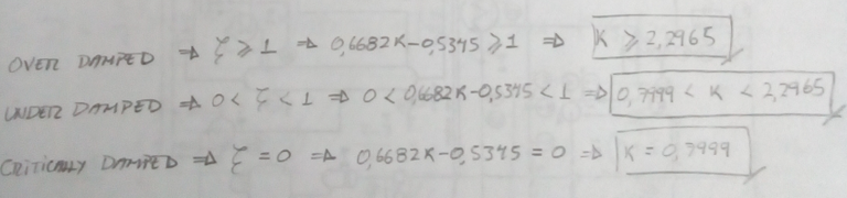
We already saw that the damped factor ζ depends on K and according to its value, we could have either an under, over, or critically damped system. In the next figure, we posed the cases and find the values range for K.
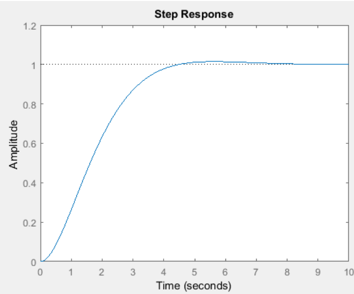
The next figure shows the system simulation for a unit step input, the student can prove this result checking out the equations that depend on K from the past figures and selecting the value K=2 for them.
Exercise 6: Magnetics Circuits
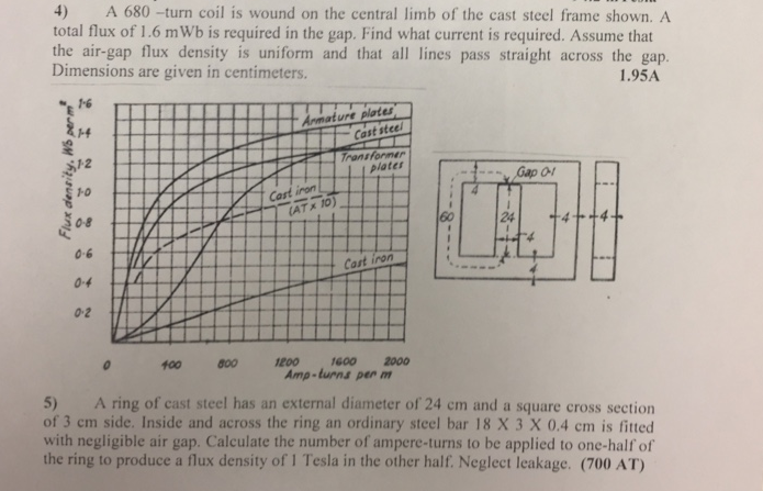
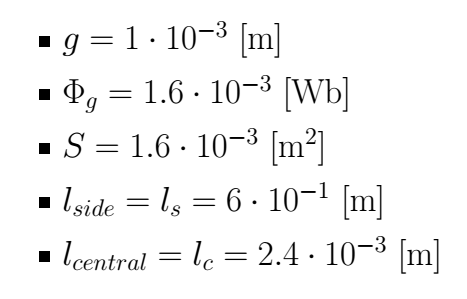
Let's assemble our prime data
The equivalent magnetic circuit is
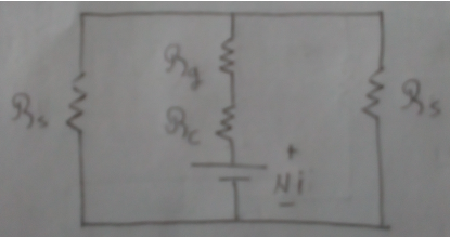
Since the central limb has the same geometry of the gab, B doesn't change, therefore Φg = Φc and Bc can be computed by
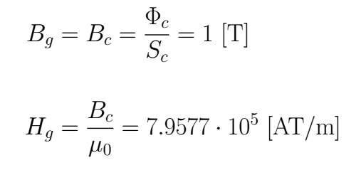
To find the Hc we need to see the graph and look at what value of H corresponds to Bc, the value is Hc=900 [Av/m].
Using the symmetry in the cast steel isn't difficult to see that Φs = Φc/2
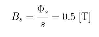
And using the graph again, we have Hs = 540 [AT/m].
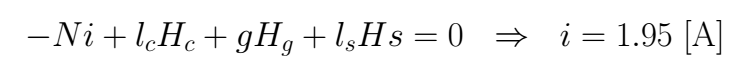
Finally, we pose the equation in the right loop
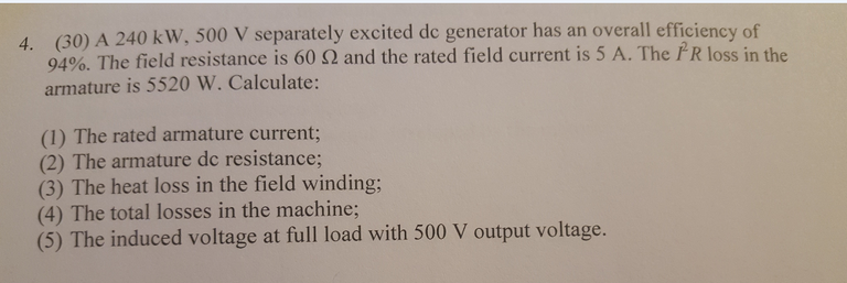
Exercise 7: DC machine
Let's draw the circuit diagram for the separately excited generator DC.
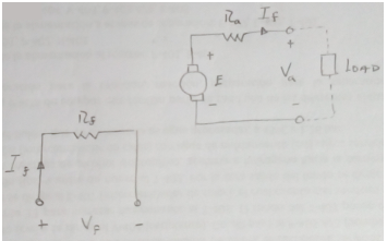
The nominal data of the DC machine in general are
- Voltage in the field circuit Vfn.
- Voltage in the armature circuit Van.
- Current in the field circuit Ifn.
- Current in the armature circuit Ian
- Output Power in the machine axis Pout in [W] or[HP]
- Mechanical Velocity in the machine axis ωn in [rad/s] or [rpm]
For this case, we have the next data
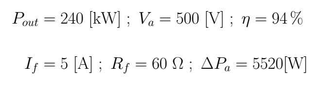
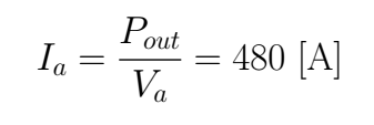
If the load is consuming its nominal power $240\cdot 10^{3}$ at nominal voltage $500$ then nominal current in the armature is
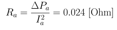
We can compute the Ra using the loss in the armature
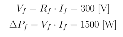
For the field, is easy to compute Vfn and then its loss
In the general case, the total loss in power is computed with the following expression
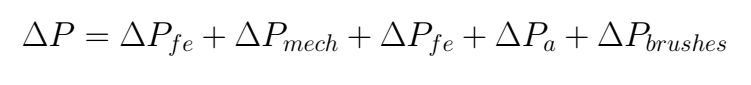
In this case, we only can compute
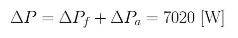
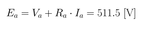
Finally, for the armature