Fourier Series + Exercise + Python Code
In my opinion, we are in front of a remarkable subject related to math for engineering. A math course that tries to teach advanced topics for engineering cannot omit The Fourier's Series because the wide range for its applications is large, a really good course for Signals and Systems should always include it as well as a mechanical vibrations course, electrical energy quality, communications, tec. Even though the statement is simple:
Decompound a periodic signal which meets the Dirichlet's conditions in a linear combination of sine and cosine functions
This treatment has to be done carefully to avoid mistakes in the calculations and in the result analysis (this is very important in engineering). Besides, these series give us a tool for the calculation of the numerical series' sum, this is possible to understand from the signal's energy making use of Parceval's theorem. It is recommended for the reader to look for alternative sources of information to the ones we offer here to complete the topics reviewed, a good book of systems and signal will be good enough. Finally is remembered that it is going to make a treatment to series and successions, therefore a review of these topics is recommended for a quick advance.
Conditions for a periodic function to have a Fourier series.
In most engineering textbooks, a function f(t) has a Fourier Series if it satisfied the following conditions
- f(t) is entirely integrable over any period.
- f(t) only has a finite number of maximums and minimus over any period.
- f(t) only has a finite number of maximums and minimus over any period.
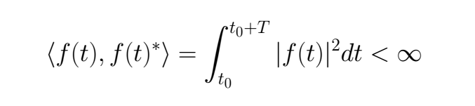
We can resume the past conditions ensuring for the existence of this integral
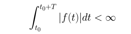
For this work we are going to regard a "stronger" condition, this is that the square norm defined for the studied function is finite, this means that the function belongs to the L² norm.
Fourier Series convergence theorem
If f(t) is piecewise smooth on the interval [t0 ≤ x ≤ t0 + T ], then the Fourier series converges to
- The function periodicity of f(t), where the function periodicity is continuous
- The one sided limits average (1/2) [ f(+x) + f(-x) ] where the periodic extention has a singularity jump.
That is to say, if the function doesn't have a singularity in its period the series is equal to the function where it is smooth. But, if there is a singularity in any point, in this the function converges to the next value (1/2) [ f(+x) + f(-x) ].
Fourier Series appearance
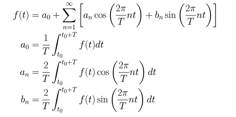
Each textbook, each teacher, each course, you can find the Fourier Series in different topology (appearance), to avoid a mess, here it will be given a simple explanation. In principle, for a period functionT we have
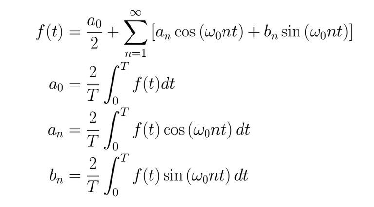
Now, let's suppose that who is writing wish to have symmetry in the integrals quotients (that all of them begin with 2/T), also, that the significant data in the integral argument is the fundamental frequency in the wave (we know that ω = 2π / T = 2π f) and finally it is known that the wave begins to repeat from the origen to forward, thus
The topology to be used will depend on the problem's features to deal with and how we want to make the calculations. For example, for math exams is convenient to choose signals whose period is multiple of π to simplify the calculations
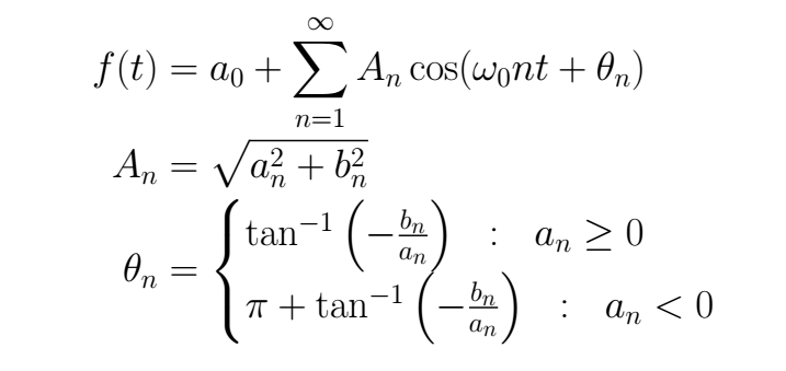
Starting from the trigonometric functions, there is another topology used in engineering that is better related to the phasors.
Another topology, with usually used to start the Fourier Series definitions is its complex form, here we are not going to go deep into the relations between these topologies because they can be found in many textbooks.
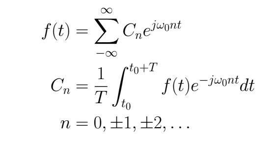
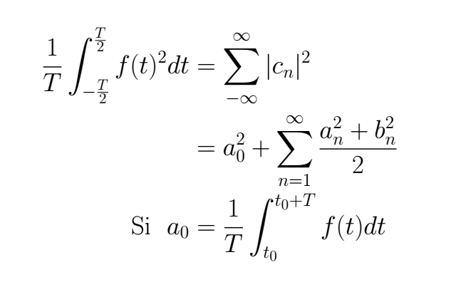
Parceval's theorem
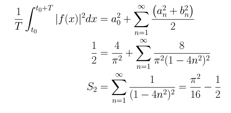
Let the following function f(t) with period T the math representation of a physical signal. In the next equation, we can see in its left side the signal's average power while in its right side is shown this power how the square absolute value sum of its Fourier Series coefficients
Now, let's do a simple exercise to understand all this theory
Exercise
- Draw the 2π periodic extention of f(x)=|sin(x)| to help you to calculate its Fourier Series, and calculate it.
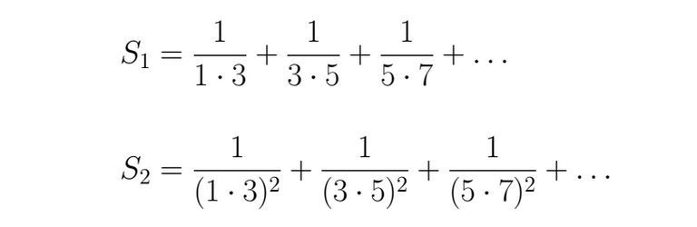
- To calculate the sum of the nex series.
It is left as an exercise to verify that the function belongs to the
A 2π periodic extension for this function which is already π periodic imply we can choose the integral limits as we wish, but in range to embrace a 2π interval. For instance, we could take into account one of the following intervals
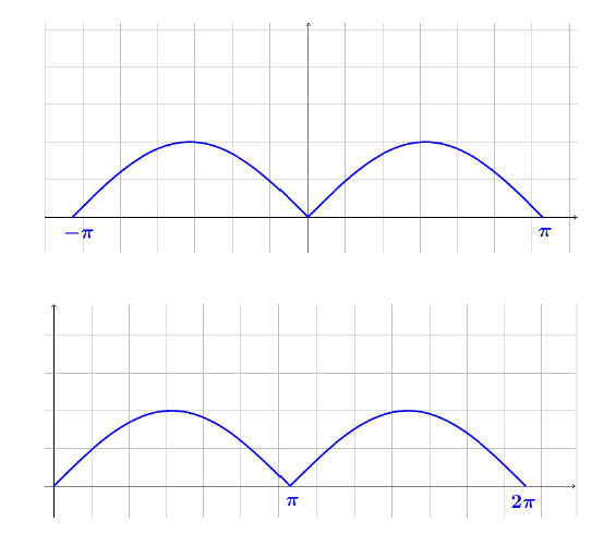
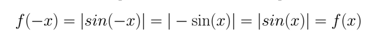
We take the first interval for the calculations. We verify first if the function is even or odd as we expect
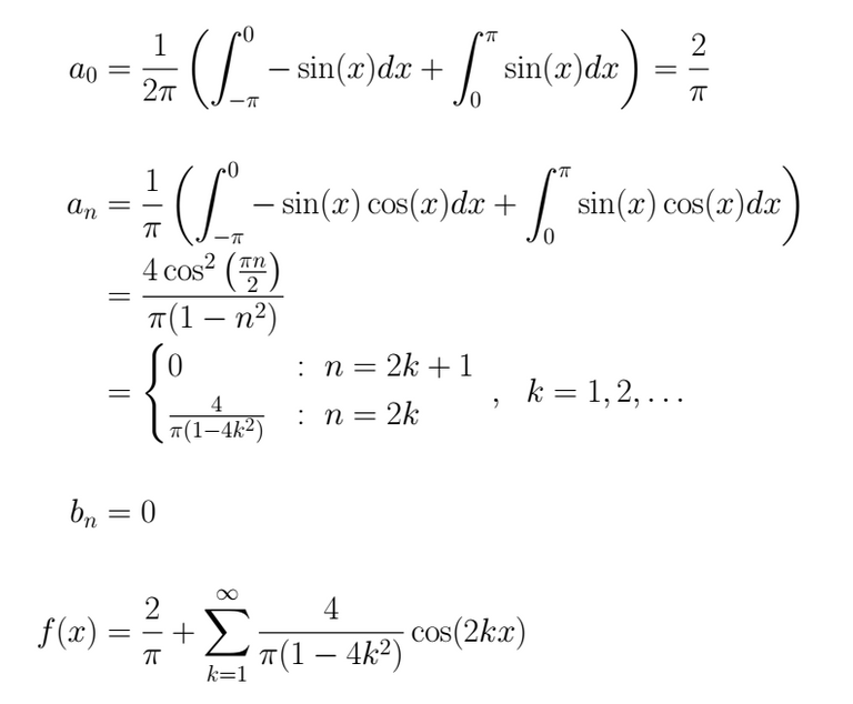
We calculate the Fourier Coefficients and we show the series
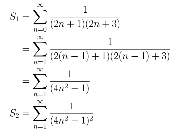
For the second part of the exercise, the first step is to find the general expression for both sums, this step can be difficult depending on the series given, for that we recommend the review of this subject for this exercise. In this particular case that we have to deal with now, for S1 we have for the denominator only odd numbers, being the second that multiple it which is followed in the odd arrangement, for S2 we have the same but squared.
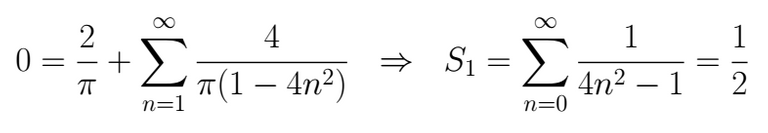
If we make x=0 in S1 we will be able to find
For S2 we think in use the Parceval identity because it adds the squared in the series coefficients, and is that what it needs.
Python code
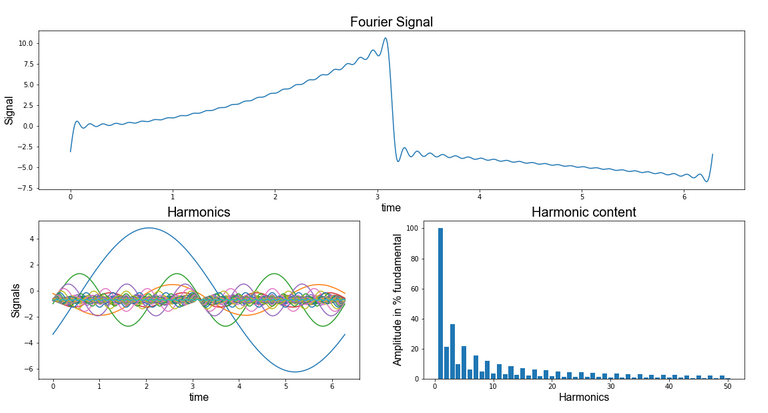
The next one is a Python code to calculate the Fourier Series of a periodic function expressed symbolically and also it shows its harmonic content.
# -*- coding: utf-8 -*-
"""
Created on Thu Aug 13 12:10:44 2020
@author: Venancio
"""
#%%
try:
from IPython import get_ipython
get_ipython().magic('clear') # to clear the terminal
get_ipython().magic('reset -f') # to reset the kernel
get_ipython().magic('matplotlib qt') # plots out line
# get_ipython().magic('matplotlib', 'inline') # plots in line
except:
pass
#%%
import numpy as np
from numpy import *
import sympy as smp
from sympy import *
import matplotlib.pyplot as plt
from matplotlib import cm
from matplotlib.ticker import LinearLocator, FormatStrFormatter
from matplotlib.gridspec import GridSpec
# from mpl_toolkits import mplot3d
import scipy as scp
from scipy.optimize import *
from scipy.integrate import *
import control as co
# import pandas as pd
# import sklearn as sk
# import math
# import os
# import tarfile
# import urllib
np.set_printoptions(precision=4, suppress=True) # number of decimals in the expre.
init_printing(use_unicode=True) # to show in pretty symboic
#%%
x , n = symbols( 'x n' )
T = 2*pi
xt = np.arange( 0 , 2*np.pi , 1e-2)
xt = np.array([ xt ])
armo = 50
#%%
## Function 1
# a0 = (1/(T))*( integrate( 1 , (x , 0 , T/2) ) +\
# integrate( -1 , (x , T/2 , T) ) )
# a0 = simplify(a0)
# an = (2/(T))*( integrate( 1*cos((2*pi/T)*n*x) , (x , 0 , T/2) ) +\
# integrate( -1*cos((2*pi/T)*n*x) , (x , T/2 , T) ) )
# an = simplify(an)
# bn = (2/(T))*( integrate( 1*sin((2*pi/T)*n*x) , (x , 0 , T/2) ) +\
# integrate( -1*sin((2*pi/T)*n*x) , (x , T/2 , T) ) )
# bn = simplify(bn)
## Function 2
a0 = (1/(T))*( integrate( x**2 , (x , 0 , T/2) ) +\
integrate( -x , (x , T/2 , T) ) )
a0 = simplify(a0)
an = (2/(T))*( integrate( x**2*cos((2*pi/T)*n*x) , (x , 0 , T/2) ) +\
integrate( -x*cos((2*pi/T)*n*x) , (x , T/2 , T) ) )
an = simplify(an)
bn = (2/(T))*( integrate( x**2*sin((2*pi/T)*n*x) , (x , 0 , T/2) ) +\
integrate( -x*sin((2*pi/T)*n*x) , (x , T/2 , T) ) )
bn = simplify(bn)
## Function 3
# a0 = (1/(T))*( integrate( sin(x) , (x , 0 , T/2) ) +\
# integrate( -sin(x) , (x , T/2 , T) ) )
# a0 = simplify(a0)
# an = (2/(T))*( integrate( sin(x)*cos((2*pi/T)*n*x) , (x , 0 , T/2) ) +\
# integrate( -sin(x)*cos((2*pi/T)*n*x) , (x , T/2 , T) ) )
# an = simplify(an)
# bn = (2/(T))*( integrate( sin(x)*sin((2*pi/T)*n*x) , (x , 0 , T/2) ) +\
# integrate( -sin(x)*sin((2*pi/T)*n*x) , (x , T/2 , T) ) )
# bn = simplify(bn)
#%%
S1, S2 = 0, 0
M1 = np.zeros( (armo , len( xt[0,:] ) ) )
ante = np.zeros( ( 1 , len( xt[0,:] ) ) )
ArC = np.zeros( ( 1 , armo ) )
nArm = np.array( [np.arange( 1 , len(M1[:,0])+1 ) ] )
# Here are created
for N in range( 1 , armo+1 ):
An = float( an.subs( n , N ).evalf() )
Bn = float( bn.subs( n , N ).evalf() )
S1 = An*cos( (2*pi/T)*N*x )
S2 = Bn*sin( (2*pi/T)*N*x )
Lda = lambdify( x , S1 , 'numpy' )
Ldb = lambdify( x , S2 , 'numpy' )
M1[[N-1],:] = ( Lda( xt )+Ldb( xt ) )
ArC[[0],N-1] = np.max( M1[[N-1],:] )
# Here are cleaned those harmonics = 0
M1 = np.round( M1 , 4 )
M1 = M1[~np.all(M1 == 0, axis=1)]
nArm2 = np.array( [np.arange( 1 , len(M1[:,0])+1 ) ] )
M2 = np.zeros( M1.shape )
# Here is created a Mtx whose rows are the harmonic sum
for N in range( 1 , len( M2[:,0] ) + 1 ):
if (N == 1):
M2[[N-1],:] = M1[0,:]
if (N > 1):
M2[[N-1],:] = M2[[N-2],:] + M1[[N-1],:]
# The Fourier Series is created
Fourier = a0 + sum(M1 , axis=0)
#%%
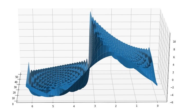
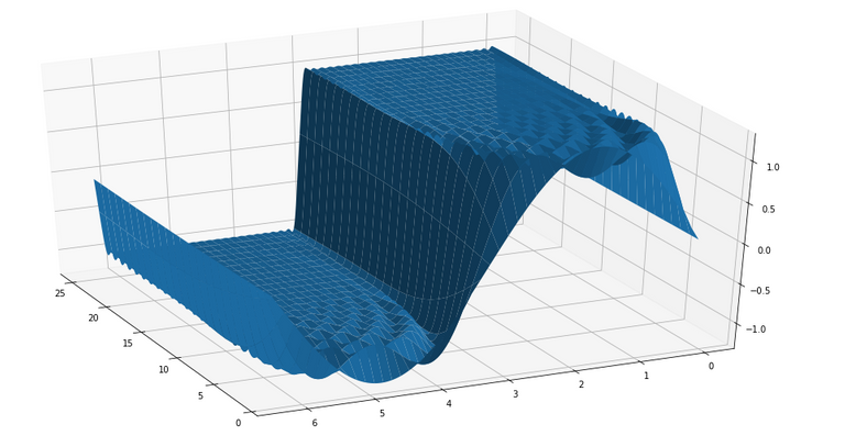
fig1 = plt.figure()
ax = fig1.gca( projection='3d' )
surf = ax.plot_surface( nArm2 , xt.T , M2.T ,
linewidth=1,
antialiased=True)
# cmap=cm.coolwarm
# Customize the z axis.
# ax.set_zlim(-1.01, 1.01)
# ax.zaxis.set_major_locator(LinearLocator(10))
# ax.zaxis.set_major_formatter(FormatStrFormatter('%.02f'))
# Add a color bar that maps values to colors.
# fig1.colorbar(surf, shrink=0.5, aspect=5)
plt.show()
#%%
fig1 = plt.figure()
plt.subplot(2,2,(1,2))
plt.plot( xt.T , Fourier.T )
plt.title('Fourier Signal' , fontdict = {'fontname': 'Arial' , 'fontsize':20} )
plt.xlabel('time' , fontdict = {'fontname': 'Arial' , 'fontsize':16} )
plt.ylabel('Signal' , fontdict = {'fontname': 'Arial' , 'fontsize':16} )
plt.subplot(2,2,3)
plt.plot( xt.T , M1.T + a0 )
plt.title('Harmonics' , fontdict = {'fontname': 'Arial' , 'fontsize':20})
plt.xlabel('time' , fontdict = {'fontname': 'Arial' , 'fontsize':16} )
plt.ylabel('Signals' , fontdict = {'fontname': 'Arial' , 'fontsize':16})
plt.subplot(2,2,4)
plt.bar( nArm.reshape(len(nArm[0,:]),) ,
( ArC.reshape(len(ArC[0,:]),) / np.max(M2[0,:]))*100 )
plt.title('Harmonic content' , fontdict = {'fontname': 'Arial' , 'fontsize':20})
plt.xlabel('Harmonics' , fontdict = {'fontname': 'Arial' , 'fontsize':16})
plt.ylabel('Amplitude in % fundamental' , fontdict = {'fontname': 'Arial' , 'fontsize':16})