am back! Hope all of you are taking good care of yourselves during these trying times...

In this article, we'll try to generate our own sounds from math functions, we'll also try to hear one of the blackhole mergers using the same technique, all at our own computers.., using our sound generation skills!

^{(This post is best viewed on Peakd.com)}

^{(Comparison of gravitational waves detected at detectors in Hanford and Livingston.)}

We'll use Python for this article.
If you haven't got it installed on your PC (which is very unlikely as it comes bundled with OS and programs many times), you can always install it, its open-source, and free.

(Website: https://www.python.org/)

1. Quick Python Installation

For installation instructions, please visit the official documentation page here: https://docs.python.org/3/using/index.html

2. Installing PyAudio and Numpy

PyAudio is a Python library that will help us generate our sounds. Installing PyAudio should be simple on Windows and Mac, its slightly tricky on Ubuntu (Linux) though.
Numpy is another Python library which has useful maths functions and other things we'll need for numerical manipulation of data.

Win / Mac
Open the terminal, and punch the following and press Enter.

pip install pyaudio

Next, we'll install numpy in a similar fashion:

pip install numpy

Ubuntu

sudo apt-get install libasound-dev portaudio19-dev libportaudio2 libportaudiocpp0
sudo apt-get install ffmpeg libav-tools
sudo pip3 install pyaudio

Now, to install Numpy:

sudo pip3 install numpy

NOTE: In Ubuntu, if pip3 is not already installed, you'll have to first install it by the command:

sudo apt-get install python3-pip

3. Writing the code

To generate sound using a function, we'll have to first write a python program, then give a function to the program, and run it.

First of all we need to import all the modules we'll be requiring in our program. We can import these any time in between the code as well, but it is a good practice to import everything in the beginning.

import pyaudio
import numpy as np

as allows us to use an acronym for the modules whenever they need to be called.

Next, we need to set up the portaudio system, for which we'll instantiate PyAudio:

pyaudio.PyAudio.open()

Defining our audio. This is the most crucial step...

samples = (np.sin(2*np.pi*np.arange(sample_rate*duration)*f/sample_rate)).astype(np.float32)

To play audio, we open a stream on the desired device with the desired audio parameters...

stream = p.open(format=pyaudio.paFloat32, channels=1, rate=44100, output=True)

After having opened the desired stream, we play the audio to the stream:

stream.write(1.0*samples)

Now, to close the streams...

stream.stop_stream()
stream.close()

Finally, we need to terminate and close our portaudio system...

p.terminate()

So, that's for the code...
Putting it all together, we get:

import pyaudio
import numpy as np

p = pyaudio.PyAudio()

samples = (np.sin(2*np.pi*np.arange(44000*2)*580/44000)).astype(np.float32)

stream = p.open(format=pyaudio.paFloat32, channels=1, rate=sample_rate,output=True)

stream.write(1.0*samples)

stream.stop_stream()
stream.close()

p.terminate()

We can make the code slightly easier to manipulate by listing all the variables together clearly.

import pyaudio
import numpy as np

p = pyaudio.PyAudio()

volume = 1.0    
sample_rate = 44100       
duration = 2.0   
f = 580.0        


samples = (np.sin(2*np.pi*np.arange(sample_rate*duration)*f/sample_rate)).astype(np.float32)

stream = p.open(format=pyaudio.paFloat32, channels=1, rate=fs, output=True)

stream.write(volume*samples)

stream.stop_stream()
stream.close()

p.terminate()

I'll at the moment not go into too much detail of the working of the code, other than the fact that the variable volume should be in the range [0.0, 1.0] (this corresponds to the volume at which the audio will be played), the variable sample_rate is the rate at which the values of sin function are sampled and played (higher the sample rate, clearer the audio), the variable duration corresponds to the duration of the sound played, and lastly variable f is the frequency of the waveform.

NOTE: Sample rate is measured in hertz (Hz). According to the Nyquist-Shannon Sampling Theorem, the sampling frequency to produce the exact original waveform should be double the original frequency of the signal. So, since the audible frequency range for humans is 20-20kHz, the sample rate is generally kept at 44kHz.
Increasing it beyond 44kHz will give no appreciable improvement in sound quality.

4. Running the code

To run the code, simply open a text editor, and paste the code in it. Then save it as a .py file.
Next, open your terminal, and run it using the command:

(Let's say the name of your file is sound.py ...)

python <location_of_sound.py>\sound.py

If the code executes without any errors, you will hear something like this:

Presently we ran the program on a simple sin wave:

But, what if we run it on something like this:

Plot	Description
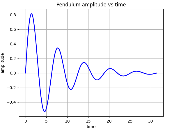	I have taken this plot from my previous article: Playing with Graphs. The function that we used there was: y = pow(1.72181, -0.25*x)*np.sin(x), let's try a similar decaying sin curve but with different parameters...

We'll have to modify our code for this function:

import pyaudio
import numpy as np

p = pyaudio.PyAudio()

volume = 1.0    
sample_rate = 22000       
duration = 4
f = 580.0        


samples = (np.sin(2*np.pi*np.arange(sample_rate*duration)*f/sample_rate)).astype(np.float32)
print(len(samples))

for i in range (len(samples)):
    samples[i] = samples[i]*pow(0.999, 0.5*i)

stream = p.open(format=pyaudio.paFloat32, channels=1, rate=sample_rate, output=True)

stream.write(volume*samples)

stream.stop_stream()
stream.close()

p.terminate()

So, what we have done essentially is that, this time, we have taken the entire array samples and multiplied each subsequent term with 0.999 raised to the power of half of its index in the array. This way we have damped the sound...so it fades away rather than staying constant.

Try fiddling with the numbers a bit, and you'll understand by experiment what actually is happening.

On running this code, we'll hear something like this:

5. One Last Experiment

In the previous example, we tried damping the sound by reducing the amplitude over time. But sound has another property, and that is its frequency.

So, can we make the sound change its frequency as time passes?

Curve	Description
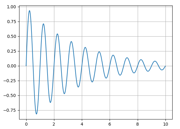	I f you look at this curve carefully, you'll find the for every 2 units we move on the horizontal axis, our curve has 2 peaks (wavelengths) i.e. frequency is constant. This is what we have done so far.
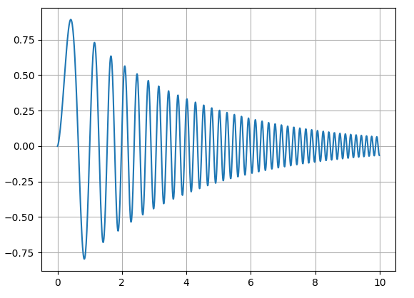	This is what we want to do now. In this case the frequency also increases with time, and hence the pitch of the sound...

Well yeah sure! Let's try:
In our previous code, the information regarding the frequency is stored in this line:

f = 580.0    

...and its value is put to use in this line:

samples = (np.sin(2*np.pi*np.arange(sample_rate*duration)*f/sample_rate)).astype(np.float32)

So, as in the damping experiment, in this experiment as well, we'll have to somehow change the value of f for each element of the array: samples.
We create a new array:

Note: The length of the new frequency matrix that will store our frequencies should be the same as the list: np.arange(sample_rate*duration)

frequency = np.zeros(len()np.arange(sample_rate*duration))
for i in range(len(frequency)):
    frequency = f*pow(1.001,0.5*i)

You can see that we have used the same trickery we used for damping sound, only this time, we are not damping it with time, but rather increasing it...
Now, to incorporate this in samples:

samples = np.zeros(len(frequency))

for i in range(len(samples)):
    samples[i] = (np.sin(2*np.pi*i*frequency/sample_rate)).astype(np.float32)

...so the pitch of the sound should increase with passage of time.
So, our final code for this experiment becomes:

import pyaudio
import numpy as np

p = pyaudio.PyAudio()

volume = 1.0    
sample_rate = 44100       
duration = 4
f = 580        

frequency = np.zeros(len(np.arange(sample_rate*duration)))

for i in range(len(frequency)):
    frequency[i] = f*pow(1.001,0.5*i)

samples = np.zeros(len(frequency))

for i in range(len(samples)):
    samples[i] = (np.sin(2*np.pi*i*frequency[i]/sample_rate)).astype(np.float32)*pow(0.999, 0.5*i)
print(len(samples))


stream = p.open(format=pyaudio.paFloat32, channels=1, rate=sample_rate, output=True)

stream.write(volume*samples)

stream.stop_stream()
stream.close()

p.terminate()

Let's try running this.
What we'll hear is a chirp like this:

(NOTE: Listen with headphones.)

Now, let's try changing the frequency f:

f = 0.1

Now, it sounds something like this:

So, earlier with f = 580 , the frequency used to start increasing starting from 580Hz, and went to higher inaudible values much before the sound ended, in the latter case, the sound starts from 0.1 Hz and builds up reaching to higher frequencies much later.

---

Time to tune our ears to the Dark monsters!

Okay, now we'll try to model the two merging blackholes using the sound released by LIGO.

LIGO:
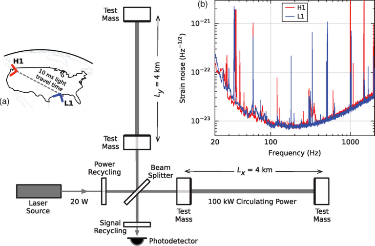
The Laser Interferometer Gravitational-Wave Observatory (LIGO) is a large-scale physics experiment and observatory to detect cosmic gravitational waves and to develop gravitational-wave observations as an astronomical tool.[1] Two large observatories were built in the United States with the aim of detecting gravitational waves by laser interferometry. These can detect a change in the 4 km mirror spacing of less than a ten-thousandth the charge diameter of a proton.

^{(Layout of the huge Michelson interferometer at LIGO)}

Blackholes are very heavy objects, Let's say we have two stellar mass blackholes (these are the ones whose masses are comparable to the mass of the Sun). Stellar mass Black holes are 5 - several tens solar masses. We take the masses of our blackholes to be 20 solar masses.

Solar Mass: Solar Mass = Mass of Sun = 2 x 10³⁰ kg.

For simplicity let's assume these to be point masses.

Let's say we have a mass attached to a string, and we are rotating the mass so that the mass remains nearly horizontal.

• When string is short: we find that we need to spin the mass faster to keep the string taught.
• When string is long: we find that even spinning the masses at a comparatively lower rate is able to keep the string taught.

So, this is also the same with gravity...
Two objects passing-by at high speeds and pulling each other at the same time will actually start orbiting each other while they continue to come closer. With reducing separation, the speed at which they orbit increases and keeps increasing till they collide. This has got to do with the conservation of angular momentum of the two objects.

So, in the case of black holes, it looks something like this:

LIGO Simulation	Diagrammatic Description
The above video shows a simulation of a merger as it would appear to the eye.	The above simulation shows the gravitational waves which are otherwise invisible and largely undetectable.

So, what we'll we trying to do is to convert these gravitational waves into audible sound waves and listen!!

There are two ways of proceeding:

1. We acquire raw gravitational wave frequency data.
2. We listen to the sound already released by LIGO and try to replicate it using our code, and learn from it. We'll take this route!

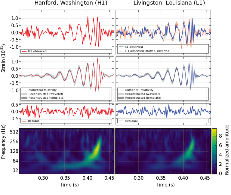
Now, that we know some blackhole basics of the basics, let's watch this ultra short video released by LIGO which contains the original "chirps" of the blackhole mergers obeserved by LIGO, and then let's try and replicate those using our knowledge of chirping in Python!

As we can clearly see in the spectrogram, the chirps start at a frequency of about 40Hz, and peak at a time roughly 0.2 seconds from impact.
Now, we have to model this sound...

But, first let's run the code for the plane sin wave that we wrote in the very beginning, but with a frequency: f = 40Hz...we need to see if this sounds good for the beginning of the chirp.

We'll run it with the following parameters:

volume = 1.0    
sample_rate = 22000       
duration = 10
f = 40.0        

Okay, this sounds decent...This should be our frequency at the start...

Now, let's try to playing more with the "damped-chirping" code that we wrote and try to model the sound given in the video above as "Natural Frequency"...

NOTE: We don't want to damp the sound, so, we'll remove *pow(0.999, 0.5*i) from the second for loop.

import pyaudio
import numpy as np

p = pyaudio.PyAudio()

volume = 1.0    
sample_rate = 88100       
duration = 10
f = 40        
a = 0.00000000000002
b = 0.000000000000000006                       
c = 0.0000000000000000000000006                            
d = 0.00000000000000000000000000000000014
e = 0.00000000000000000000000000000000000000000006

frequency = np.zeros(len(np.arange(sample_rate*duration)))

for i in range(len(frequency)):
    frequency[i] = float(f+ a*i + b*pow(i,3) + c*pow(i,5) + d*pow(i,7) + e*pow(i,9))

samples = np.zeros(len(frequency))

for i in range(len(samples)):
    samples[i] = (np.sin(2*np.pi*i*frequency[i]/sample_rate)).astype(np.float32)
print(len(samples))


stream = p.open(format=pyaudio.paFloat32, channels=1, rate=sample_rate, output=True)

stream.write(volume*samples)

stream.stop_stream()
stream.close()

p.terminate()

Running the above code will give us a sound like this one which I recorded:

I have tried to model the rising frequency using a polynomial of degree 9.

This is the best I could achieve after hours of tweaking the code and trying different techniques.

The limitation is not theoretical, but rather of the technique I have used to achieve this.

NOTE: What I have tried to do in the code above is to model the frequency curve using a polynomial of degree 9. But, I realised that, we have the following limitations in this technique:

1. We need to use higher degree polynomials, 9 is just not sufficient.
2. Using higher and higher degree polynomials creates a lot of disturbance in the sound (which is very much clear if we listen to the plain 40 Hz tone followed by the last one that we just made).
3. Increasing the sampling rate (sample_rate) reduces it to some extent, but all sampling rates are not support and give errors sometimes. Plus, there is a limit beyond which the computer cannot store data...since, increasing the rate means that the computer need to create, then store that much amount of data before it can play the sound and delete it. That's a limitation of the Python data-type we are using, and of Python itself.

So, yes there can definitely be better ways of doing it...so keep playing with the code!

But, this is at least a step towards becoming perfect! Playing with the code more, and trying a different function instead (of the polynomial), or trying a polynomial of an even higher degree may give us better sound output with closer resemblance to the original.

The values of the coefficients a, b, c, ...may have a physical significance and can tell us about the masses of the merging blackholes, provided we can get accurate values of them!

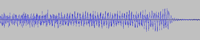
BEFORE WE CLOSE! : Do you remember the first image in this article?...especially the waveform of the gravitational waves?
If you try to record the audio output from your program, and visualise it as a waveform using suitable software / techniques, you'll find that it has a similar waveform.

Here, I have done it for you:

Is it really similar? If not we can compare and learn from the differences, for eg. we need a sharper, more dramatic end and a near linear initial phase which is not there in our waveform. Secondly, our waveform has a lot of noise which shows up in this as erratic wiggle of the sin wave.

---

Credits

All images and media used in this article are my intellectual property unless otherwise stated.
I am thankful to the following sources:

1. Comparison of gravitational wave observations..., Source: Wikipedia.org | CC by 3.0 License.
2. LIGO schematic diagram: Wikipedia.org | CC License.
3. Youtube Video: Two Black Holes Merge into One, Author: LIGO Lab Caltech MIT (Educational video)
4. Youtube video-2 : Warped Space-time around a ... , Author: LIGO Lab Caltech MIT (Educational video)
5. Youtube Video: Comparing Chirps of ..., Author: LIGO Lab Caltech MIT (Educational video)

---

Thanks, hope you enjoyed listening to Blackholes and mimicking their noises!!
See you later,
M. Medro