Laboratory Project: Logistic Sequences
In this video I go over some mathematics for a change after going all year working on my game changing #AntiGravity Part 6 video. In this video I look at the “Laboratory Project” on Logistic Sequences; note that laboratory projects are very interesting math projects at the end of some sections in my calculus book titled Early Transcendentals by James Stewart. The logistic sequence is defined by the logistic difference equation:
Current population = (a constant k) * (previous population)*(1 – previous population)
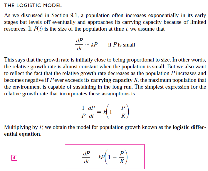
Note that this equation is similar to the logistic differential equation which I covered earlier and is given by the following formula.
Population growth = (a constant k) * population (1 – population / carrying capacity K)
The logistic sequence involves individual discrete values for the population size and is often preferred for modeling insect populations where mating and death occur periodically. In this project I take a look at modeling the logistic equation using Microsoft Excel spreadsheet to compare how the populations change with changing initial populations and constant k. Interestingly for some values of k there appears to be a leveling off of the population into 1 or more branches. But for other larger values of k the model gives very chaotic and spread out values for the population. The link to the Excel sheet is listed below so make sure to download it and play around with the logistic sequence model!
Watch Video On:
- 3Speak: https://3speak.tv/watch?v=mes/jaeagukv
- Odysee: https://odysee.com/@mes:8/laboratory-project-logistic-sequences:0
- BitChute: https://www.bitchute.com/video/cdcfELetKCUN/
- Rumble: https://rumble.com/v20tlra-laboratory-project-logistic-sequences.html
- DTube: https://d.tube/#!/v/mes/QmXMjLCaqccd943gDLsmzWBCfqi8gLyrt63q5dnsYSfdg7
- YouTube: https://youtu.be/OqP7Gmv96Ec
Download Video Notes:
- PDF Notes: https://1drv.ms/b/s!As32ynv0LoaIh8N8XBPGW5vi1TjDKw
- Excel File: https://1drv.ms/x/s!As32ynv0LoaIh8N-Iy9FpTaG99wgJA?e=vQl3RQ
View Video Notes Below!
Download these notes: Link is in video description.
View these notes as an article: https://peakd.com/@mes
Subscribe via email: http://mes.fm/subscribe
Donate! :) https://mes.fm/donate
Buy MES merchandise! https://mes.fm/store
More links: https://linktr.ee/matheasyReuse of my videos:
- Feel free to make use of / re-upload / monetize my videos as long as you provide a link to the original video.
Fight back against censorship:
- Bookmark sites/channels/accounts and check periodically
- Remember to always archive website pages in case they get deleted/changed.
Recommended Books:
- "Where Did the Towers Go?" by Dr. Judy Wood: https://mes.fm/judywoodbook
Subscribe to MES Truth: https://mes.fm/truth
MES Links Telegram channel: https://t.me/meslinksJoin my forums!
- Hive community: https://peakd.com/c/hive-128780
- Reddit: https://reddit.com/r/AMAZINGMathStuff
- Discord: https://mes.fm/chatroom
Follow along my epic video series:
- #MESScience: https://mes.fm/science-playlist
- #MESExperiments: https://peakd.com/mesexperiments/@mes/list
- #AntiGravity: https://peakd.com/antigravity/@mes/series
-- See Part 6 for my Self Appointed PhD and #MESDuality breakthrough concept!- #FreeEnergy: https://mes.fm/freeenergy-playlist
- #PG (YouTube-deleted series): https://peakd.com/pg/@mes/videos
NOTE #1: If you don't have time to watch this whole video:
- Skip to the end for Summary and Conclusions (if available)
- Play this video at a faster speed.
-- TOP SECRET LIFE HACK: Your brain gets used to faster speed!
-- MES tutorial: https://peakd.com/video/@mes/play-videos-at-faster-or-slower-speeds-on-any-website- Download and read video notes.
- Read notes on the Hive blockchain #Hive
- Watch the video in parts.
-- Timestamps of all parts are in the description.Browser extension recommendations:
- Increase video speed: https://mes.fm/videospeed-extension
- Increase video audio: https://mes.fm/volume-extension
- Text to speech: https://mes.fm/speech-extension
--Android app: https://mes.fm/speech-android
Laboratory Project: Logistic Sequences
Laboratory Projects
Recall from my earlier videos in which I would go over very interesting math applications in the form of "laboratory projects" which are included in the end of some sections in my Calculus book (Early Transcendentals by James Stewart).
Logistic Sequences
A sequence that arises in ecology (study of organisms and their environment) is defined by the logistic difference equation:
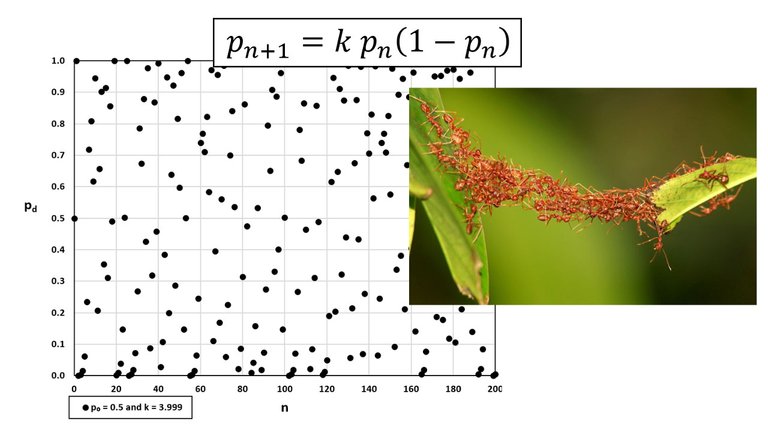
pn+1 = k pn (1 - pn)
where pn measures the size of the population of the nth generation of a single species.
To keep the numbers manageable, pn is a fraction of the maximal size of the population, so 0 ≤ pn ≤ 1.
Notice that the form of this equation is similar to the logistic differential equation from my earlier video.
https://peakd.com/mathematics/@mes/differential-equations-population-growth-logistic-equation
Retrieved: 10 June 2019
Archive: http://archive.fo/R6QrJ
The discrete (individually separate and distinct) model - with sequences instead of continuous functions - is preferable for modeling insect populations, where mating and death occur in a periodic fashion.
An ecologist is interested in predicting the size of the population as time goes on, and asks these questions:
- Will it stabilize at a limiting value?
- Will it change in a cyclical fashion?
- Or will it exhibit random behavior?
Write a program to compute the first n terms of this sequence starting with an initial population p0, where 0 < p0 < 1.
Use this program to do the following.
Task 1:
Calculate 20 or 30 terms of the sequence for p0 = 1/2 and for two values of k such that 1 < k < 3.
Graph the sequences.
Do they appear to converge?
Repeat for a different value of p0 between 0 and 1.
Does the limit depend on the choice of p0?
Does it depend on the choice of k?
Task 2:
Calculate terms of the sequence for a value of k between 3 and 3.4 and plot them.
What do you notice about the behavior of the terms?
Task 3:
Experiment with values of k between 3.4 and 3.5.
What happens to the terms?
Task 4:
For values of k between 3.6 and 4, compute and plot at least 100 terms and comment on the behavior of the sequence.
What happens if you change p0 by 0.001?
This type of behavior is called chaotic and is exhibited by insect populations under certain conditions.
Solutions:
Solution to Task 1:
Calculate 20 or 30 terms of the sequence for p0 = 1/2 and for two values of k such that 1 < k < 3.
Graph the sequences.
Do they appear to converge?
Repeat for a different value of p0 between 0 and 1.
Does the limit depend on the choice of p0?
Does it depend on the choice of k?
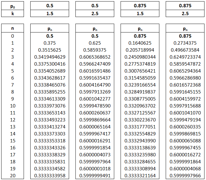
I have tabulated 20 terms for the sequences with the following values for p0 and k.
MES Note: You can download my Excel sheet in the following link.
https://1drv.ms/x/s!As32ynv0LoaIh8N-0itIkBrT5E2YMw
Retrieved: 11 June 2019
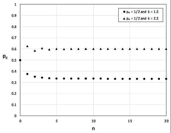
Plotting the sequences all together, the following chart is shown:
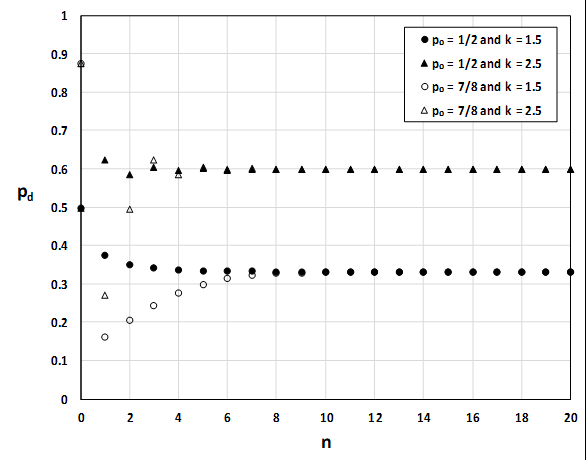
For p0 = 1/2 the sequence converges to about 1/3 for k = 1.5 and about 0.60 for k = 2.5.
For p0 = 7/8 the sequence still converges to about 1/3 for k = 1.5 and about 0.60 for k = 2.5.
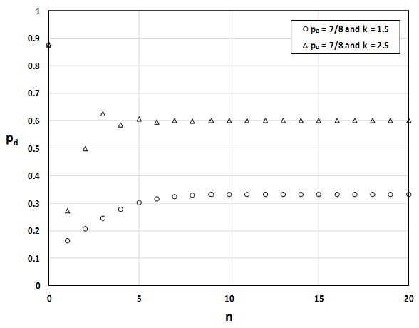
The limit of the sequence seems to depend on k, but not on p0.
Solution Task 2:
Calculate terms of the sequence for a value of k between 3 and 3.4 and plot them.
What do you notice about the behavior of the terms?
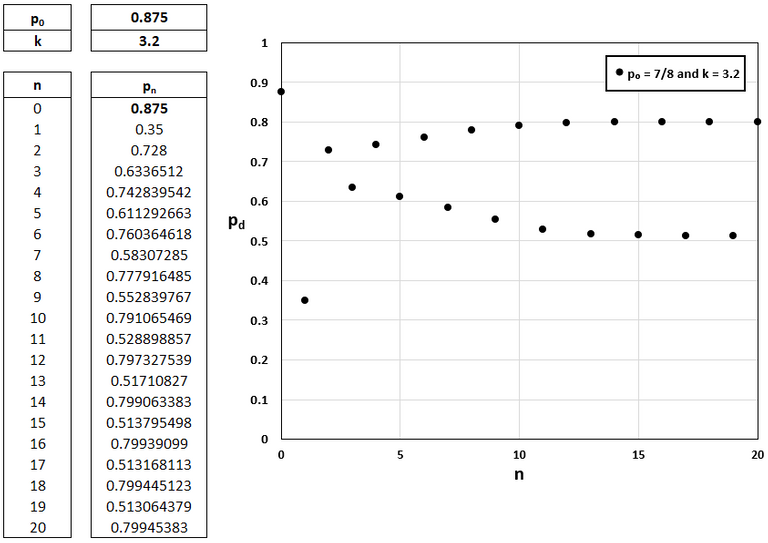
Plotting in the same Excel sheet from above, and selecting p0 = 7/8 and k = 3.2, it seems that the terms of the sequence fluctuate between two values (about 0.5 and 0.8 in this case).
Solution to Task 3:
Experiment with values of k between 3.4 and 3.5.
What happens to the terms?
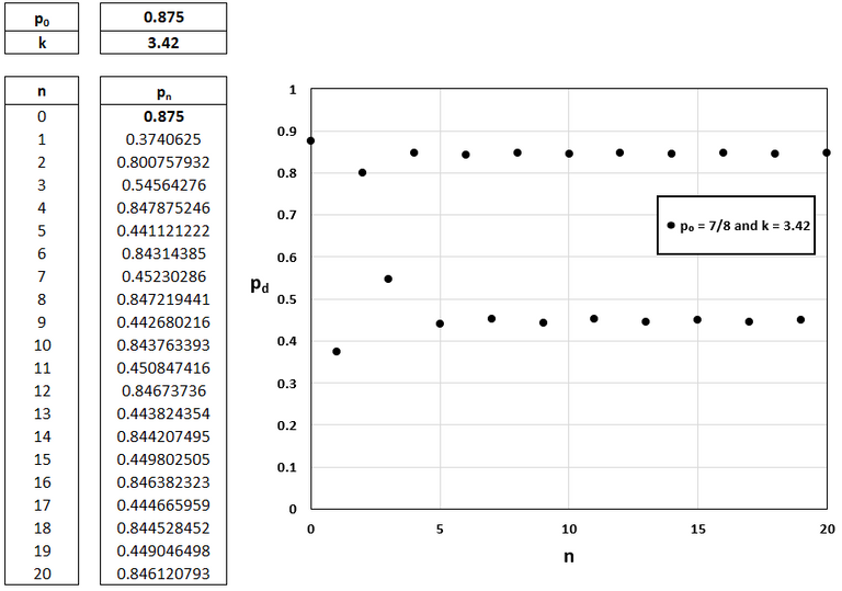
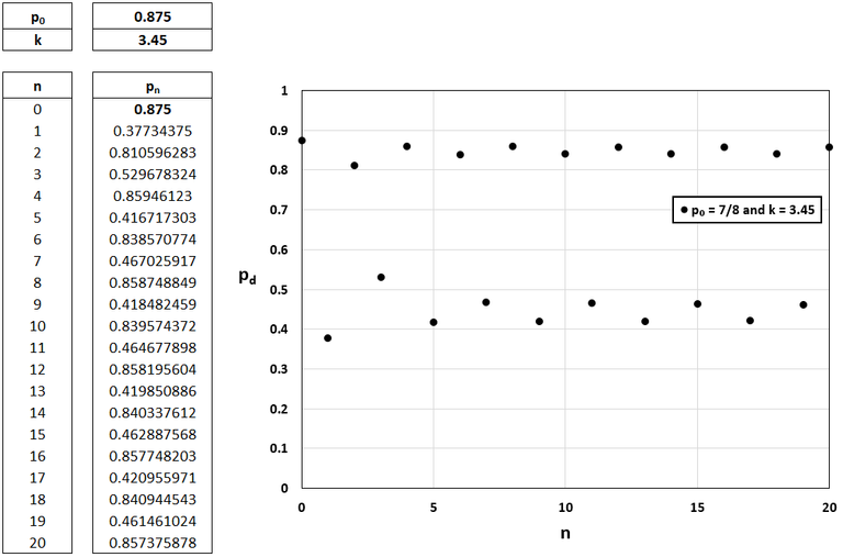
For p0 = 7/8 and k = 3.42 or 3.45 it appears the terms eventually fluctuate between four values.
Note that for the following chart for k = 3.42 my calculus book states that the pattern persists into these four distinct "branches" even after 1000 terms which in that case the first and third terms in the pattern differ by only 2 x 10⁻⁹-9 while the first and fifth terms differ by only 2 x 10⁻¹⁰.
These terms are 0.44980, 0.84638, 0.44466, 0.84452, 0.44904, etc.
This pattern is seen more clearly when k = 3.45.
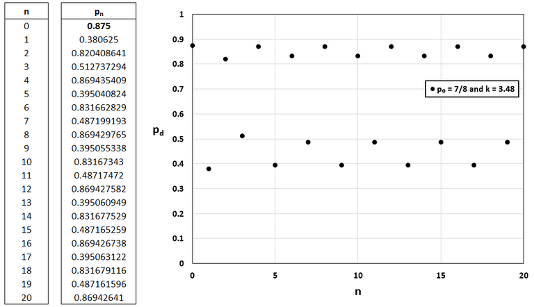
For p0 = 7/8 and k = 3.48 the sequences fluctuates about the terms 0.395, 0.832, 0.487, 0.869, 0.395, etc.
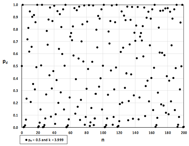
Solution to Task 4:
For values of k between 3.6 and 4, compute and plot at least 100 terms and comment on the behavior of the sequence.
What happens if you change p0 by 0.001?
This type of behavior is called chaotic and is exhibited by insect populations under certain conditions.
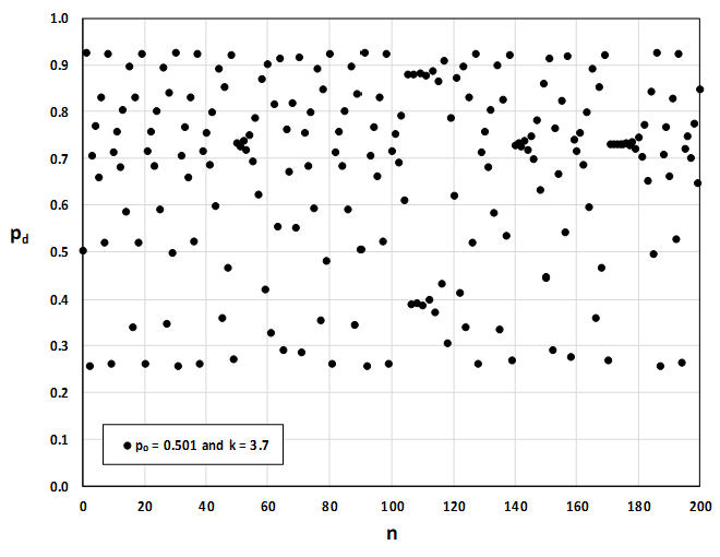
The chart for p0 = 0.5 and k = 3.7 is shown below.
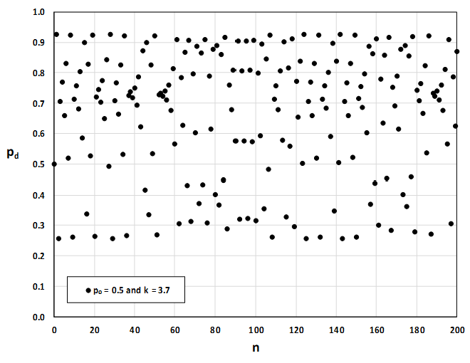
Increasing p0 by 0.001 changes the graph completely.
For p0 = 0.75 and k = 3.9 the chart is once again changed completely by modifying p0 by 0.001.
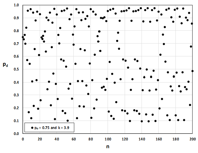

As k increases the values are spread out vertically with extreme values getting close to 0 and 1.
There seem to be some fleeting patterns in these graphs, but on the whole they are certainly very chaotic.