Chaotic Real-Valued Sequences By Skew Tent Map

almost 4 years ago

0. Note

This is the first assignment from my Masters Applied Digital Information Theory Course which has never been published anywhere and I, as the author and copyright holder, license this assignment customized CC-BY-SA where anyone can share, copy, republish, and sell on condition to state my name as the author and notify that the original and open version available here.

1. Introduction

The chaos theory is a field of study in mathematics that studies the behaviour of dynamical system. Rober L. Devaney stated a system can be chaotic if it is sensitive to initial value, topologically mixing, and have a dense periodic orbit. The theory was summarized by Edward Lorenz. Although the system was highly determined by the initial value, in the end the sequence is unpredictable. Chaos exist in many natural system such as the climate and whether. In the field of computer science, it's applied to generate random values.

2. Tent Map

The tent map can be formulated as t = x/c for 0 ≤ x < c and t = (1-x)/(1-c) for c ≤ x ≤ 1 where:

c = critical point

x = initial value

t = tent map (next value for sequence)

For example c = 0.5 with x from 0 to 1:

Figure 1. Tent Map 1.jpg

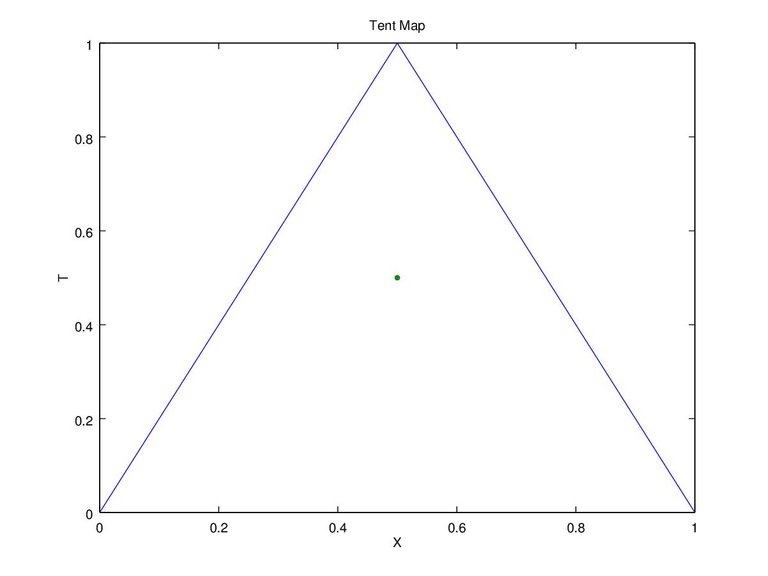
Figure 1. Tent Map 1

Figure 1 is based on the equation that the value would range from 0 to 1, and when “x” reached the critical point, the value of “t” will equals to 1. It is up to us to decide the critical point, as in Figure 2 shows if “c” equals to 0.2. Another information is if “x” equals to 0 or 1 the end result will be 0, thus using this value is not recommended.

Figure 2. Tent Map 2.jpg

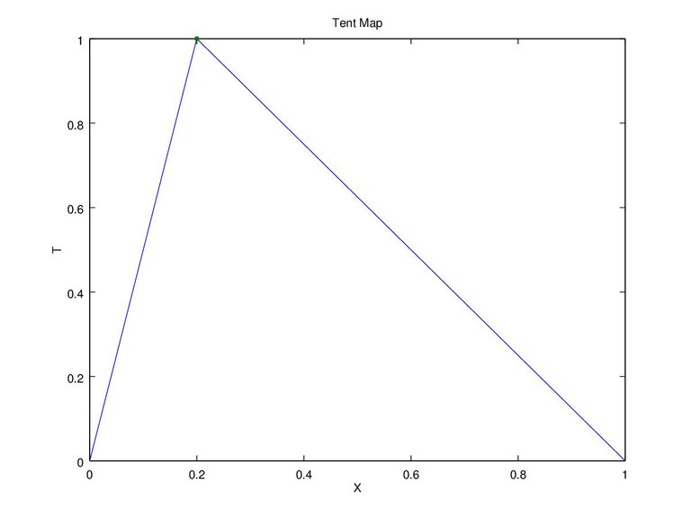
Figure 2. Tent Map 2

3. Chaotic Sequence

In some areas the tent map equation is used to generate chaotic sequence, here t(n) = x(n+1). The equation would turn into x(n+1) = (x(n))/c for 0 ≤ x(n) < c and x(n+1) = (1-x(n))/(1-c) for c ≤ x(n) ≤ 1. Why the equation is stated differently? So the value of x(n+1) will never exceed 1. For example if “c = 0.4” and “x = 0.5” and use the first equation “x(n)/c = 0.5/0.4 = 1.25”. That won't do so we use “1-x(n)/1-c = 1 - 0.5 / 1 - 0.4 = 0.5/0.6 = 0.833”. Another example “c = 0.7” and “x = 0.4” which we can't use the second equation “1-x(n)/1-c = 1 - 0.4 / 1 - 0.7 = 0.6/0.3 = 2” but we use “x(n)/c = 0.7/0.4 = 0.571”.

As stated in the chaos theory the next sequence “x(n+1)” is highly dependable on the initial value “x(n)” (x(2) depends on x(1), x(3) depends on x(2), etc), as we plot the sequences it will looked unpredictable.

3.1 For “x” equals to 0 and 1, and “c” equals to 0.5

Figure 3a. x-0 and c-0.5.jpg

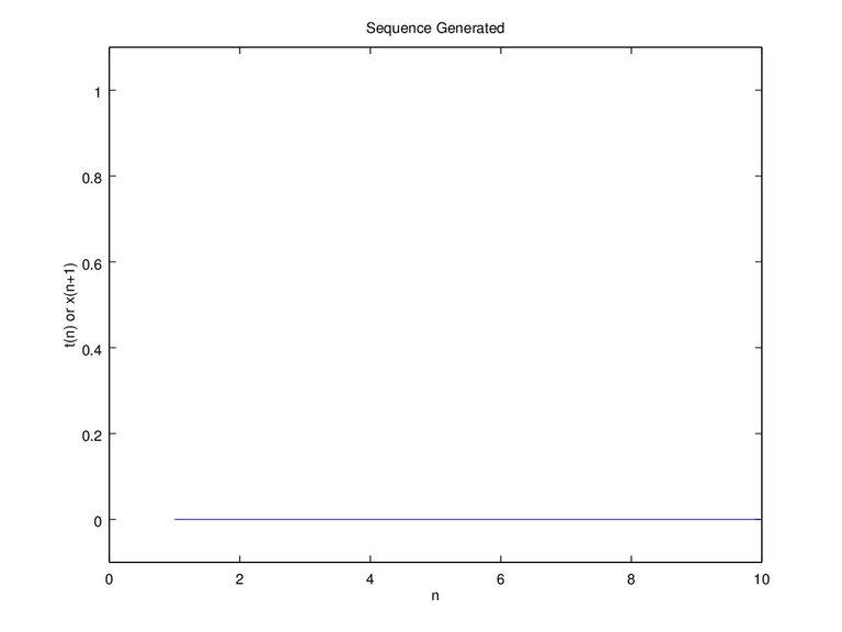
Figure 3a. image x(1) = 0

Figure 3b. x equals c.jpg

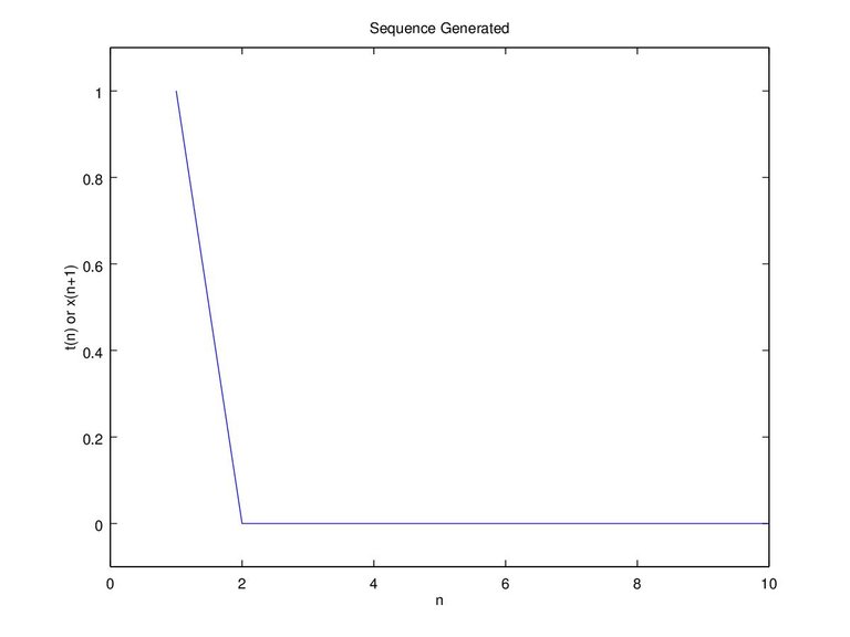
Figure 3b. image x = c

Figure 3 is only plotted to the 10th “n” because the result is obvious. For x(1) (initial) equals to 0, x(2) = 0/c = 0 and for x(1) x(2) = (1-1)/(1-c) = 0/(1-c) = 0. Once the value is zero, the next value will always be zero, and for x(1) equals to c x(2) = c/c = 1, x(3) = (1-1)/(1-c) = 0. When “x” reaches critical point “c” it will result to 1, and once the next value “x(n+1)” equals to 1 the next value “x(n+2)” will result to 0, and once it reaches to 0 the next value will always be 0. With the explanation above we can see that it's not recommended to use a critical point “c” equals to 0.5. In Figure 4b when “c = 0.5” it's susceptible for “x” in reaching “c”. On the 54th “n” “x(n) = c” and “x(n+1) = 1”, then the next result will always be 0.

Figure 4a. x-0.2 and c-0.5 tent.jpg

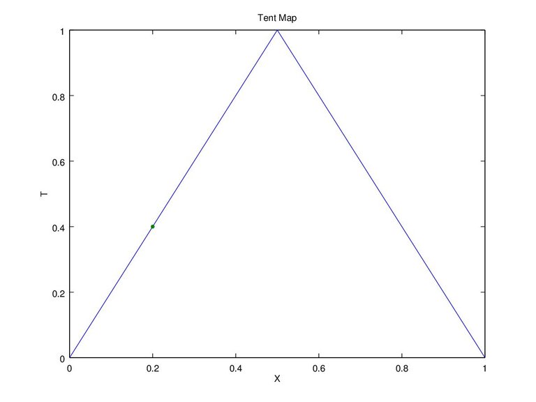
Figure 4a. Tent map x(1) = 0.2 and c = 0.5

Figure 4b. x-0.2 and c-0.5.jpg

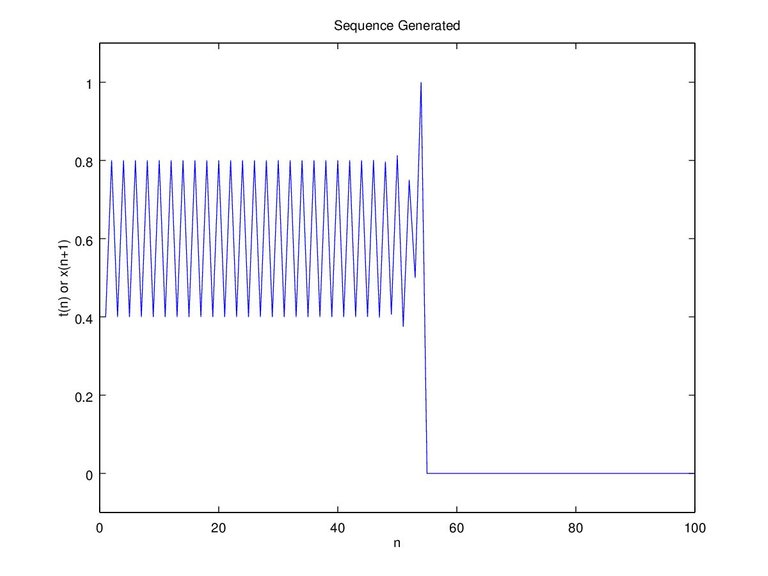
Figure 4b. Sequence x(1) = 0.2 and c = 0.5

3.2 For “c” equals to 0.6 and x = 0.3 and 0.8

Figure 5a shows that when “c” equals to 0.6, “t” will have the same value when “x” equals to 0.3 and 0.8. Thus the sequence generated at Figure 5b will be the same. At the same time it is shown the sequence will be continuous.

Figure 5a. x-0.3 0.8 and c-0.6 tent.jpg

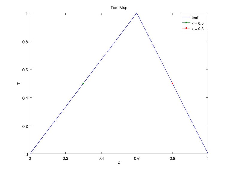
Figure 5a. Tent Map of c = 0.6 and x = 0.3 and 0.8

Figure 5b. x-0.3 0.8 and c-0.6.jpg

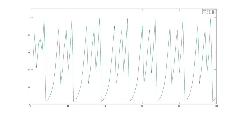
Figure 5b. Sequence x(1) = 0.3 and 0.8 (no difference)

3.3 Sensitivity to Initial Value

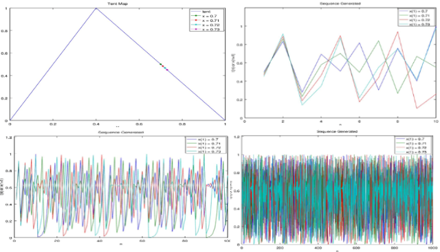
The chaos theory stated that it is sensitive to initial value, just a slight change can totally change the whole sequence. For example “c = 0.4” and we'll try “x” with initial value of 0.7, 0.71, 0.72, 0.73 on Figure 6 and “x” with initial value of 0.7111, 0.71111, 0.711111, 0.7111111 on Figure 7.

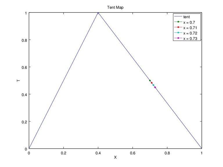
Figure 6a. x-0.7 0.71 0.72 0.73 and c-0.4 tent.jpg

Figure 6a. Graph c = 0.4 and x(1) = 0.7, 0.71, 0.72, 0.73 tent map

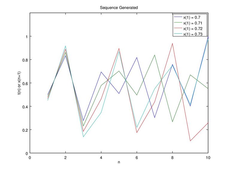
Figure 6b. x-0.7 0.71 0.72 0.73 and c-0.4 n-10.jpg

Figure 6b. Graph c = 0.4 and x(1) = 0.7, 0.71, 0.72, 0.73 up to 10 sequence

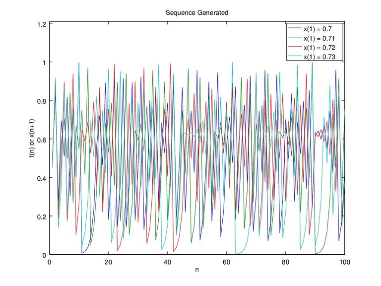
Figure 6c. x-0.7 0.71 0.72 0.73 and c-0.4 n-100.jpg

Figure 6c. Graph c = 0.4 and x(1) = 0.7, 0.71, 0.72, 0.73 up to 100 sequence

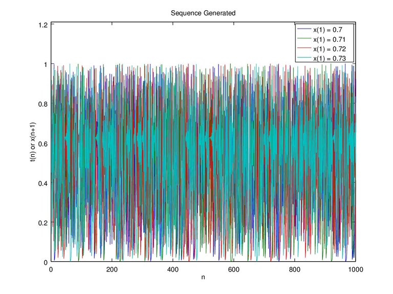
Figure 6d. x-0.7 0.71 0.72 0.73 and c-0.4 n-1000.jpg

Figure 6d. Graph c = 0.4 and x(1) = 0.7, 0.71, 0.72, 0.73 up to 1000 sequence

On Figure 7 we tried even more extreme which we plot of each initial value with a difference of 0.0001, 0.00001, 0.000001, and 0.0000001. There seems to be no difference on up to the 10th sequence, but the sequences finally deviated on the 15th “n” sequence for 0.7111 and 0.71111, then followed up by the other initial values that have smaller difference.

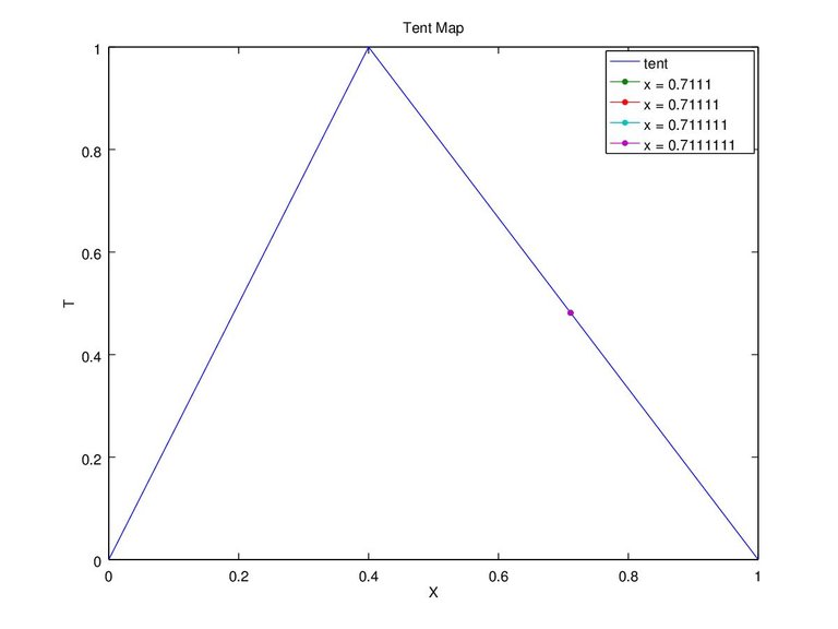
Figure 7a. x-0.7111 0.71111 0.711111 0.7111111 and c-0.4 tent.jpg

Figure 7a. Graph c = 0.4 and x(1) = 0.7111, 0.71111, 0.711111, 0.7111111 tent map

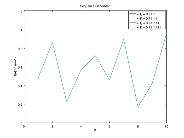
Figure 7b. x-0.7111 0.71111 0.711111 0.7111111 and c-0.4 n-10.jpg

Figure 7b. Graph c = 0.4 and x(1) = 0.7111, 0.71111, 0.711111, 0.7111111 up to 10 sequence

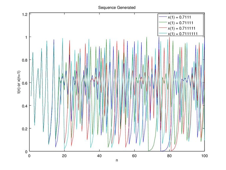
Figure 7c. x-0.7111 0.71111 0.711111 0.7111111 and c-0.4 n-100.jpg

Figure 7c. Graph c = 0.4 and x(1) = 0.7111, 0.71111, 0.711111, 0.7111111 up to 100 sequence

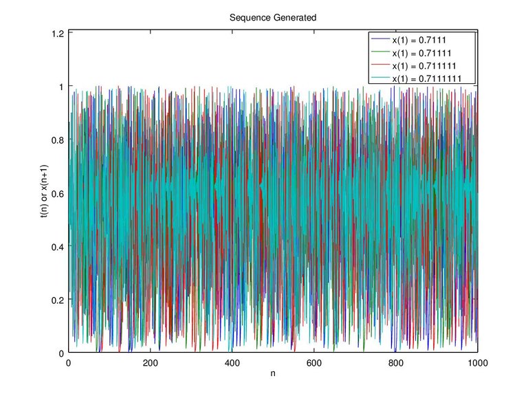
Figure 7d. x-0.7111 0.71111 0.711111 0.7111111 and c-0.4 n-1000.jpg

Figure 7d. Graph c = 0.4 and x(1) = 0.7111, 0.71111, 0.711111, 0.7111111 up to 1000 sequence

Even with small difference it's still unpredictable on the 100th sequence, let alone the 1000th sequence. This proofs the sensitivity to initial values (where the “x” starts).

3.4 Distributions of the sequences

On this section we will see the distribution of value from 0 to 1, specifically from 0, 0.01, 0.02 ~ 1. Only 0 to 1 because the sequence is formulated to not go below 0 and go above 1. The histogram on Figure 8 shows the distribution of value with critical point “c” of 0.4 and initial value “x(1)” of 0.7. This time we produce a sequence as much as “n = 1000000” (million) (the more the sequence the better). Plotting that much data cannot be seen in one graph, in other word it's not visible, but with histogram we can see what and how much the values contained in the sequence.

Figure 8. x-0.7 hist distribution.jpg

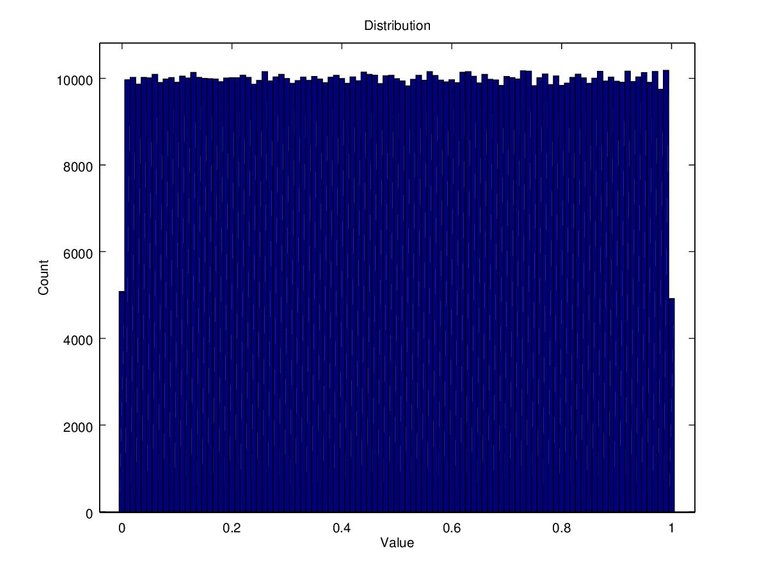
Figure 8. Data count on x(1) = 0.7, c = 0.4, n = 1000000

Figure 8 shows that there is around 10000 data with a value of 0.1, 0.2, and so on. The hist() function works by rounding, for example the value of 0.1111 will be rounded to 0.1, and the value of 0.15 rounded to 0.2. Then the value is counted up (how many 0.1s there is) and a distrubution histogram was graphed. Finally it can be said that the distribution of data is uniformed since the amount of data for each value is almost the same.

4. Conclusion

We can conclude that the chaos sequence is formed by previous value like a memory system. Since it's very sensitive to initial value, the further the sequence becomes more unpredictable. The theory is a simple application of the natural system for example the weather. We can predict the weather maybe for a month, beyond that it's likely miss prediction. The course of whether is determined by its starting point, the wrong initial value will lead to the wrong prediction. On the other hand the more accurate the initial value and the formula, the longer the validity of the prediction. Since the unpredictable outcome of this chaos theory, in computer it can be also applied for creating random values. On this simulation the distribution of the skew tent to the chaotic sequence, we found it to be uniformed.

5. Source Code

The source code is written in “m file” that could run on Matlab or Octave alike. It is a function which can be run as “stcsfp(xo,c,N)” where “xo = initial value”, “c = critical point”, and “N = number of sequence”. For example the plotted graph above we run by “stcsfp(0.7,0.4,1000000)”, but we can delete function if it seems inconvenient by deleting the 1st line and use it as regular script. The graphs above are done by few modifications of the code, but here on Code 1 resides the pure source code.

function t = stcsfp(xo,c,N)

% === TENT MAP === %

X = 0:.1:1;

for n = 1:11
 if X(n) >= 0 && X(n) < c
  T(n) = X(n)/c;
 elseif X(n) >= c && X(n) <=1
  T(n) = (1-X(n))/(1-c);
 else
  printf("x initial must be from 0 to 1");
 end
end

% === MAIN CALCULATION === %
x(1) = xo;

for n = 1:N
 if x(n) >= 0 && x(n) < c
  t(n) = x(n)/c;
  x(n+1) = t(n);
 elseif x(n) >= c && x(n) <=1
  t(n) = (1-x(n))/(1-c);
  x(n+1) = t(n);
 else
  printf("x initial must be from 0 to 1");
 end
end

%Plot Tent Map%
figure
plot(X, T, xo, t(1));
title("Tent Map");
xlabel("X");
ylabel("T");
%legend("fill this in")

%Plot Sequence%
figure
plot(t);
title("Sequence Generated");
xlabel("n");
ylabel("t(n) or x(n+1)");
ylim([-0.1 1.1]);
%legend(["fill this in"]);
%xlim([1 20])

%Plot Histogram%
figure
hist(t, 0:.01:1);
title("Distribution");
xlabel("Value");
ylabel("Count");
xlim([-0.1 1.1]);

Code 1. Skew Tent Chaotic Sequence Program

Mirrors

math engineering chaos random assignment

0.000

0 comments