hhee I am back again!!

In this article, we'll look at some basic curve fitting techniques and the Python code to do the same.

^{(This post is best viewed on Peakd.com)}

Something that we are very interested in and have been since ages is predicting the future!!...It could be predicting the stock market, or maybe the prices of crypto-currencies in the coming future, or it may be a due to some scientific need like predicting how a rocket will function at a later stage for which data is not available...and so on..

Another interesting application can be in astronomy where we can gather data ,giving clues to the trajectory of an asteroid or a Near Earth Object and predict whether or not it has chances of impacting our planet in the future.

...there are numerous such applications of curve fitting....so hold tight!

1. Getting started

Some terminologies:

1. Extrapolation: This the more common of the other terms. It pertains to extending a trend beyond available data points to guess the situation in the unknown range.
2. Interpolation: this is the act of trying to find values between two known data points.
3. Regression: is the general process of fitting a curve to a given data-set, or more simply to find a pattern in a given dataset.

Regression (According to Merriam Webster):
a functional relationship between two or more correlated variables that is often empirically determined from data and is used especially to predict values of one variable when given values of the others.

So, generally the order in which the above operations are performed is:
Obtain Data ---> Perform regression ---> Proceed to Interpolation or extrapolation

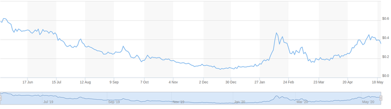
In this article, I'll try to use the current Hive Dollar Price in US Dollar trend obtained from: https://www.marketwatch.com/investing/stock/hive/charts?countrycode=ca

To start with, I save the data as a .txt file which I can directly read through my Python program.

Hive USD Chart
--------------
Range: 17 Jun 2019 - 18 May 2020, Step Size = 28 days

Day Price(USD)
0   0.50
1   0.45
2   0.33
3   0.25
4   0.18
5   0.18
6   0.13
7   0.10
8   0.14
9   0.31
10  0.18
11  0.26
12  0.40

NOTE: In this .txt file, the indices 1, 2, 3... are the number of steps starting from 17 June 2019, each step is 28 days long. So, 0 means 17 June 2019, 1 means 15 July 2019...and so on.

2. Storing our Data

Types of data files:

1. Text:
   files starting with .txt. These are the most commonly used files for importing numerical data, but they are not very popular. They are easy to create and edit. They are the least standardized, so you can make them in whichever you need provided, you can program your code to import them.
2. CSV (Comma-Separated Values):
   files ending with a .csv. These are more popular than text files. Programs like Excel allow importing data as CSV. But, for us they should be as easy to import as a text file since we'll be writing our own program. Just creating a .txt file with the "comma-separated" data and renaming it to .csv format should do.
3. SQLite and other standard database files:
   These are used for more advanced data storing purposes like in Firefox and other browsers...File extension: .sqlite3, .sqlite, .db

In our program, we'll try importing data from .txt file and a .csv file and then carry on with whichever is easier to program for!

Let's name our files data.txt and data.csv respectively...Then, we have:

Contents of data.txt	Contents of data.csv
0 0.50 1 0.45 2 0.33 3 0.25 4 0.18 5 0.18 6 0.13 7 0.10 8 0.14 9 0.31 10 0.18 11 0.26 12 0.40	0,0.50 1,0.45 2,0.33 3,0.25 4,0.18 5,0.18 6,0.13 7,0.10 8,0.14 9,0.31 10,0.18 11,0.26 12,0.40

NOTE: I have left the first lines of both the files empty.

Now, open a text editor, copy the contents and save them with the filenames specified.

At present, I don't know whether .csv even works, I have tried importing data from .txt file though. I guess, csv should be as easy...but let's see...as we proceed, we should come to know what works and what doesn't!!

3. Let's start coding!

If you are not sure whether Python and Numpy are installed on your machine, please check the point 1 and 2 (we don't need PyAudio this time) in my previous post: Mimicking Blackhole Murmurs

Reading / Importing data stored in external files.
We'll start programming now...!

• Import Python library: OS, and Numpy.

import os
import numpy

• Now, let's say the address of our file is <location>, then we'll open the file as:

fileData = file.open("<location>", "r")

NOTE: fileData is a variable that I have created, it can be named anything.

BEST PRACTICES: the use of Camel Case is a good practice while naming variables. Camel-Case means that the first letter of every word barring the first be capitalised. For example, if I want to name a variable: "My great variable", I'll name it as: myGreatVariable, this way it is easier to read.

|
|
|
|
|
|
|
|
|
|
|
|
.
You probably know more about camelCase than you think:

eBay

μTorrent

...that's all "camelCase"!!

Now, what we want to do is to read the text / csv file using our program and
store its data in an array. We do it using the following:

for line in fileData:
    line = fileData.readlines()
    print(*line)

So, our complete code becomes:

import os
import numpy as np

fileData = open("<location>/data.txt", "r")

for line in fileData:
    line = fileData.readlines()
    print(*line)

On running it, we get the following:
Output:

0 0.50
 1 0.45
 2 0.33
 3 0.25
 4 0.18
 5 0.18
 6 0.13
 7 0.10
 8 0.14
 9 0.31
 10 0.18
 11 0.26
 12 0.40

Now, we have a list by the name line, we can access elements of the list by:
(For example, let's say we want to print the 5^th element...)
print(*line[4])

NOTICE: we have used 4 as the index and NOT 5, because python starts indexing from 0.

Full Code

import os
import numpy as np

fileData = open("<location>/data.txt", "r")

for line in fileData:
    line = fileData.readlines()
    
print(line[4])

Output:

5 0.18

Now, we'll assign the first column of the data i.e. 1, 2, 3, 4, 5, 6, 7, 8, 9, 10, 11, 12 to a new 1-dimenasional array x, and the right column to an array y which will again be 1-D...
...and after that, we'll try to plot it using matplotlib like we did in the post: Playing With Graphs and Functions

Full Code:

import os
import numpy as np
import matplotlib.pyplot as plt

fileData = open("<location>/data.txt", "r")

for line in fileData:
    line = fileData.readlines()

print(*line)

x = np.zeros(13)
y = np.zeros(13)

for i in range(13):
    x[i], y[i]= line[i].split( )
ax = plt.subplot()
ax.plot(28*x,y, "ob", linestyle="solid")

plt.grid(True)
plt.title("Hive Price Chart")
ax.set_xlabel("Time (days)")
ax.set_ylabel("Price in USD")

plt.show()

NOTE: You may need to install Matplotlib using python pip install matplotlib, if not already installed.

Output:

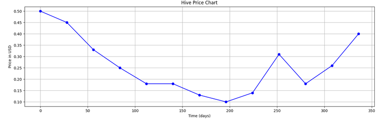
You can compare this with original Hive price chart which we had taken from the net.

txt or csv ?!
Well, we have seen the code for importing data from a .txt file, the process of importing data from a csv is same, only change the file address and make it point to data.csv, and make this minor change in split() function arguments:
x[i], y[i]= line[i].split(",")
So, since .csv is more accepted in the math world, we'll use it for the rest of the article.

Alright, now let's proceed for regression.

4. Start Regressing?

Regression is of different types:

1. Linear Regression: fit a linear curve (straight line) to the data.
2. Multi-linear Regression: fit a n-dimensional "plane" to the data?! For this, the data itself has to be n-dimensional i.e. it should be dependent upon more that one independent variables.
3. Non-linear Regression: fit a non-linear curve to the data.
4. Polynomial Regression: fit a polynomial to the data.

We'll not go into the details of theories and proofs but just stay on the practical side of the things.

A) Linear Regression

Let's say the equation of a straight line is: y = a₀ + a₁*x + c + e , where e = error, c = y-intercept.

Then, we need to find the coefficients: a0, a1 which are a₀, a₁ respectively.

We have the following equations which I am not going to prove!

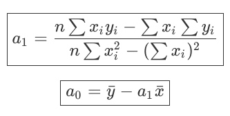
NOTE: here n = number of data points available.

Symbol	Description
	Average of all x values
	Average of all y values

So, now we just need to write a piece of code to do these two operations and we'll get the eqn for the straight line fitted to our data...

Full Code:

import os
import numpy as np
import matplotlib.pyplot as plt

fileData = open("<location>data.csv", "r")

for line in fileData:
    line = fileData.readlines()

print(*line)

x = np.zeros(len(line))
y = np.zeros(len(line))

for i in range(len(line)):
    x[i], y[i]= line[i].split(",")

sumXY = 0
sumX = 0
sumY = 0
sumX2 = 0

for i in range(len(line)):
    sumXY += x[i]*y[i]
    sumX += x[i]
    sumY += y[i]
    sumX2 += pow(x[i],2)

n = len(line)

xavg = sumX / (len(line))
yavg = sumY / (len(line))

print("sumX, sumY, sumXY, sumX2, xavg, yavg, n", sumX, sumY, sumXY, sumX2, xavg, yavg, n)

a1 = ((n * sumXY) - (sumX * sumY))/((n * sumX2) - pow(sumX,2))
a0 = yavg - (a1 * xavg)

y2 = a0 + a1 * x

print(a1, a0)

ax = plt.subplot()
ax.plot(28*x,y, "ob", linestyle="solid")
ax.plot(28*x, y2, "ob", linestyle="solid", color="g")
plt.grid(True)
plt.title("Hive Price Chart")
ax.set_xlabel("Time (days)")
ax.set_ylabel("Price in USD")

plt.show()

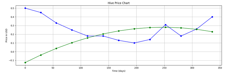
Output:

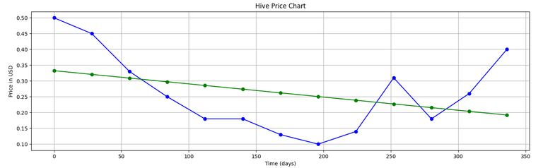
(The green line shows the linear fit given by our program...)

B) Polynomial Regression

Now that we know what the linear fit looks like, let's dive into a polynomial fit straight away...so we'll know how they differ.

Now, if we wabt to fit a second-order polynomial like this:

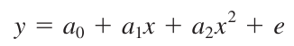
... to our data, then the algorithm to be followed is:

Algorithm for Polynomial Regression
Polynomial Regression involves the following equations being solved using the technique of Gauss Elimination.

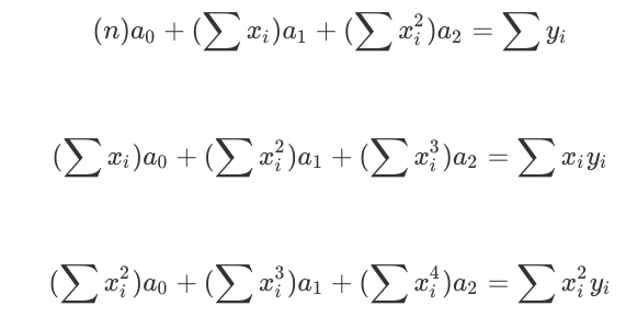
These equations can be written in matrix form as follows:

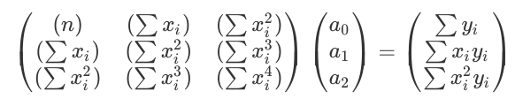
This matrix equation can now be solved using Gauss Elimination as illustrated below...

B1. Quick Review of Gauss Elimination

Steps	Description
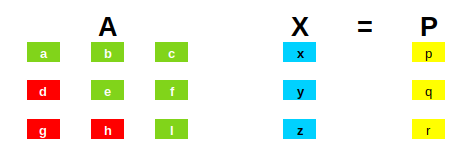	Let's say we have our matrix equations in this form. (AX = P)
We need to find the values of x, y and z (bascially the matrix X) which satisfy(s) these.	Now, X= A-1 P
For a while we'll only consider the matrices A and P, and use the elementary row operations to make the red cells of the matrices 0...whatever operations are performed on A are also performed on P simultaneously. After having performed the operations, we get the following:
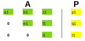	This is also commonly referred to as the elimination step. (This representation is often called: Augmented Matrix)
Now, we can substitute the values starting from the last row, for eg: z = r1 / i1, the values of z can now be substituted into row 2, and we'll get the value of y which along with z can then be substituted in row one to get the value of x.	This step is often referred to as back-substitution.

The Python code for Gauss elimination will look something like this:

import numpy as np 

data = input("Please enter the data in the form of a string of length 16(seperator = <space>): ")

data = list(data.split( ))

status = 0
for i in range(100):
    if(len(data) == i*(i+1)):
        status = 1
if(status == 0):
    raise ValueError('Please enter a valid matrix (with n rows, n+1 columns, n < 100)')

n = int(np.sqrt(len(data)))
data_m = np.zeros((n,n+1))

print(data)

k=0
for j in range(n):
    for i in range(n+1):
        data_m[j,i] = data[k]
        k+=1

print("Initial augmented matrix = \n", data_m)

# Elimination
for j in range(1,n):
    #print("LOOP-j:", j)
    for k in range(j,n):
        #print("     LOOP-k:", k)
        factor = data_m[k,j-1] / data_m[j-1,j-1]
        for i in range(n+1):
            #print("         LOOP-i:", i, "| ", data_m[k,i])
            data_m[k,i] = format(data_m[k,i] - factor*data_m[j-1,i], '7.2f')
            #print("-->",data_m[k,i])

print("Matrix after elimination = \n", data_m)

# Back Substitution
solution = np.zeros(n)

for j in range(n-1, -1, -1):
    subtractant = 0
    for i in range(n-1,-1,-1):
        subtractant = subtractant + solution[i] * data_m[j,i] 
    solution[j] = (data_m[j,n] - subtractant)/data_m[j,j]
print("Solution matrix:\n", solution)

NOTE: I have written this code in such a way, that the user doesn't need to worry about anything, just feed in the initial Augmented Matrix, and the program will automatically identify the order and solve the equations for you!
One can solve a maximum of a 100 equations simultaneously using this, for more the program will need to be tweaked a bit!

So, let's take a simple matrix equation:

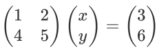
Then, our Augmented matrix simpy becomes:

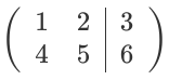
Solving these simple set of equations on paper, gives us the solution: x = -1, y = 2.
Now, running our program, and punching the values of elements of the Aug. matrix as: 1 2 3 4 5 6, ...and we get the following output:

Please enter the data in the form of a string of length 16(seperator = <space>): 1 2 3 4 5 6
['1', '2', '3', '4', '5', '6']
Initial augmented matrix = 
 [[1. 2. 3.]
 [4. 5. 6.]]
Matrix after elimination = 
 [[ 1.  2.  3.]
 [ 0. -3. -6.]]
Solution matrix:
 [-1.  2.]

B2. Back to Polynomial Regression

...continuing from where we left...

Now that we know Gauss Elimination, our task is pretty simple!

1. First, we find the values of the following: n, sumX, sumX2, sumX3, sumX4, sumY, sumXY, sumX2Y ...in a fashion similar to the code we wrote for Linear Regression.
2. Next, we write the augmented matrix, and solve using our Gauss Elimination algorithm...and hence, find the values of the coefficients: a0, a1, a2. That's it!! Hurray!

Full Code:

import os
import numpy as np
import matplotlib.pyplot as plt

# Function to sum the elements of an array
def sum(a):
    sum = 0
    for i in range(len(a)):
        sum += a[i]
    return sum

fileData = open("<location>/data.csv", "r")

for line in fileData:
    line = fileData.readlines()

print(*line)

x = np.zeros(len(line))
y = np.zeros(len(line))

for i in range(len(line)):
    x[i], y[i]= line[i].split(",")

sumX = sum(x)
sumX2 = sum(pow(x,2))
sumX3 = sum(pow(x,3))
sumX4 = sum(pow(x,4))
sumY = sum(y)
sumXY = sum(x*y)
sumX2Y = sum(pow(x,2)*y)

print(x,y)
print("sumX, sumX2, sumX3, sumX4, sumY, sumXY, sumX2Y", sumX, sumX2, sumX3, sumX4, sumY, sumXY, sumX2Y)

n = 3

data_m = np.zeros((n,n+1))

#Explicitly Defining the Augmented Matrix
data_m[0,0] = n
data_m[0,1] = sumX
data_m[0,2] = sumX2
data_m[0,3] = sumY
data_m[1,0] = sumX
data_m[1,1] = sumX2
data_m[1,2] = sumX3
data_m[1,3] = sumXY
data_m[2,0] = sumX2
data_m[2,1] = sumX3
data_m[2,2] = sumX4
data_m[2,3] = sumX2Y

print("Initial augmented matrix = \n", data_m)

# Elimination
for j in range(1,n):
    #print("LOOP-j:", j)
    for k in range(j,n):
        #print("     LOOP-k:", k)
        factor = data_m[k,j-1] / data_m[j-1,j-1]
        for i in range(n+1):
            #print("         LOOP-i:", i, "| ", data_m[k,i])
            data_m[k,i] = format(data_m[k,i] - factor*data_m[j-1,i], '7.2f')
            #print("-->",data_m[k,i])

print("Matrix after elimination = \n", data_m)

# Back Substitution
solution = np.zeros(n)

for j in range(n-1, -1, -1):
    subtractant = 0
    for i in range(n-1,-1,-1):
        subtractant = subtractant + solution[i] * data_m[j,i] 
    solution[j] = (data_m[j,n] - subtractant)/data_m[j,j]
print("Solution matrix:\n", solution)

y2 = solution[0] + solution[1]*x + solution[2]*pow(x,2)

ax = plt.subplot()
ax.plot(28*x,y, "ob", linestyle="solid")
ax.plot(28*x, y2, "ob", linestyle="solid", color="g")
plt.grid(True)
plt.title("Hive Price Chart")
ax.set_xlabel("Time (days)")
ax.set_ylabel("Price in USD")

plt.show()

Output:

C) Extrapolation

Now, let's say we need to fing the price (in USD) of hive on June 1, 2020...that is at day 350. So, basically we need to find value of y at x=350 which should be easy. We can simply add the following line of code before plt.show() in the codes for linear and polynomial interpolation:

Code to be inserted:
(For Linear Regression)

ax.plot(350, a0 + (a1 * 12.5), "ro")

(For Polynomial Regression of order 2)

ax.plot(350,(solution[0] + solution[1]*12.5 + solution[2]*pow(12.5,2)), 'ro')

Linear	Polynomial
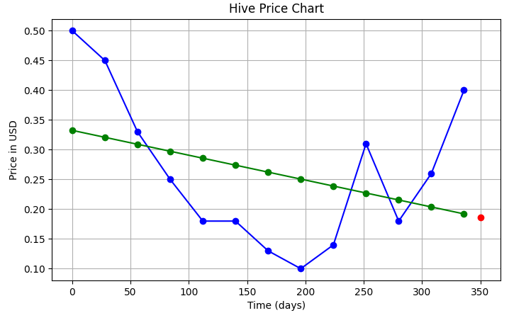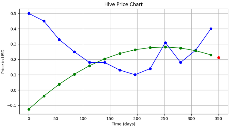Price (on Jun 1, 2020) = 0.18619 $	Price (on Jun 1, 2020) = 0.21608 $

So, you can see the different price predictions of Hive that we got from the two methods.
But, we can make our predictions better by using higher order polynomials to fit our curve...(currently we used a quadratic equation).

---

This post has already become quite lengthy due to all the code!! We'll see how to write the code for higher order polynomial regression in the next part to this series...you can of-course try writing the code yourself!!

...and maybe you can also create a Discord Bot for your Discord Server, that can predict the Hive price using regression!!

---

Credits

Unless otherwise stated, all media used in this article are my intellectual property.

I am thankful to the following sources:

1. Cover Picture: Pixabay, Pixabay License : Free for Commercial Use
2. Camel-Case Illustration: Wikipedia , CC BY SA-4.0
3. iPhone Logo: Wikipedia , CC BY SA-4.0

References

1. Wikipedia: camel case