COMMUNICATION PHYSICS: Quantization Errors, Digital Signals, Multiplexing, And How Signals Travel.

almost 4 years ago

Greetings, everyone. This is a follow-up on a series of posts I started some months ago on Communication physics, where I discussed the growth of the internet and mobile phone network. In those series of posts as well, I explained the concept of radio communication; AM and FM, the way radio waves travel, and finally on digital communications. To really understand and connect with this concluding part of the series, kindly check COMMUNICATION PHYSICS and ANALOGUE METHOD OF MODULATION: Radio and Telephone Systems.

So, in this new post, I will be explaining the errors of quantization in communication, digital signals, multiplexing, and mobile phones. So, what is it about quantization errors?

^{The simplest way to quantize a signal is to choose the digital amplitude value closest to the original analog amplitude. This example shows the original analog signal (green), the quantized signal (black dots), the signal reconstructed from the quantized signal (yellow) and the difference between the original signal and the reconstructed signal (red). The difference between the original signal and the reconstructed signal is the quantization error and, in this simple quantization scheme, is a deterministic function of the input signal. Gregory Maxwell, CC BY 3.0}

QUANTIZATION ERRORS

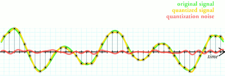
Reconstructed signals may be distorted if quantization levels are too widely spaced. Several samples that may have been slightly different in the original signal could be given the same value when the signal is reconstructed. The difference between the original sample and the reconstructed sample has the same effect as noise in analogue signals – it affects the amplitude. The difference in amplitude between the two signals – the original and the reconstructed – is a measure of the ‘noise’. The signal-to-noise ratio is better as the samples get bigger. For small samples, the ratio is very small.

There is a very simple technique which overcomes this potential problem. Instead of all quantization levels being equal, a non-linear scale is adopted. The process is called companding. In a figure showing an example of companding similar to that used in a sound recording; the first 32 levels are equal but very close together; the next 16 are also equal but slightly further apart than the first 32. Above these, there are 16 more equal levels which are slightly further apart again. This scheme continues for higher levels and is duplicated for negative samples, giving a total of 256 quantization levels. Each sample could be encoded as an 8-bit word (2⁸ = 256).

^{The DBX 566 stereo tube audio compressor. Andyzweb, CC BY-SA 3.0}

DIGITAL SIGNALS AND BIT RATES

An analogue signal would be described by its “frequency range, such as that for a radio station. This term has no meaning for a digital signal. Instead, we describe a digital signal by the number of bits – binary digits – per second.

To calculate the bit rate, we need to know the sampling rate and the number of quantization levels. The sampling rate is the number of samples every second. The levels determine the binary code and the number of ‘bits per sample’ required.
So the bit rate is given by:

Bit rate = (sampling rate) × (number of bits per sample)

The medium through which a signal travels will place a limit on the maximum frequency and on the maximum bit rate. I will look at this in more detail later in the post.

EXAMPLE

Calculate the bit rate for a signal which has a sampling rate of 8 kHz and where 16 quantization levels have been used.

ANSWER

The sampling rate is 8000 per second.
16 quantization levels can be coded by a 4-bit binary number because 16 = 2⁴
So:

bit rate = (sampling rate) × (number of bits/sample) = 8000 × 4

The bit rate for the signal = 32 000 bits per second.

BANDWIDTH OF DIGITAL SIGNALS

The bandwidth of a digital signal depends on the ‘mode’ of transmission. Let’s start thinking about what seems straightforward at first; that is, to send a series of 1’s and 0’s, rather like the signal. The 1’s and 0’s are a series of pulses, ideally ‘square’ pulses with very short transition times between 1 and 0.

In a diagram of a simple ‘square wave’ signal, there is a pattern of alternating 1’s and 0’s. This looks very simple but when such a signal is examined on a spectrum analyzer it is observed that it is far from simple, especially when it’s compared with a spectrum of a pure sine wave signal.

The sine wave spectrum contains only one peak corresponding to the frequency of the signal. The square wave signal contains many peaks, each gradually getting smaller. Looking carefully, it can be seen that the spectrum includes only odd harmonics (f, 3f, 5f, 7f, etc.)

(The spectrum can be explained using a mathematical technique first developed by the French mathematician Baron Jean Baptiste Joseph Fourier (1768-1830), called Fourier analysis. Fourier showed that any periodic signal can be made up by adding together a simple pure sine wave signal and some of its harmonics.)

If a square wave is actually made up of all these different components then its bandwidth is theoretically huge. However, in practice, we can get away with using a far narrower bandwidth. The minimum bandwidth is calculated from the time period for a single bit. If this time is t seconds, then the bandwidth has a lower limit given by:

frequency bandwidth Δf ≥ 1/t

The use of the minimum bandwidth effectively filters out all the harmonics and only allows the fundamental frequency signal through. This means that the signal at the receiver looks like a pure sine wave.

This is not a problem because the original pattern of 1’s and 0’s is still preserved in the received signal. It is very simple to ‘regenerate’ the original signal electronically using a circuit called a Schmitt trigger. The bandwidth in practice is thus determined by the period of a single bit.

^{Comparison of the action of an ordinary comparator (A) and a Schmitt trigger (B) on a noisy analog input signal (U). The green dotted lines are the circuit's switching thresholds. The Schmitt trigger tends to remove noise from the signal. FDominec, CC BY-SA 3.0}

For example, the telephone systems use a bit length of 2 to 3 μs. At 2 μs this means that the bandwidth necessary to transmit would be ½ μs^-1, which is 500 kHz (0.5MHz) or 500 kilobits per second. This is quite a large bandwidth. It would not be possible to send such a signal down an ordinary telephone connection which is just a pair of copper wires. Modems manage to overcome this using a different way of sending a digital signal. Different radio stations can share the same band because each has its own carrier frequency. The carrier frequencies are spaced out so that the stations do not overlap and interfere with each other. AM stations transmit using a bandwidth of 8 kHz.

MULTIPLEXING

I have shown different ways of transmitting information. The next question is how can you send more than one signal along a telephone cable at the same time? Alternatively, how do modern communication satellites handle thousands of telephone calls at a time? Multiplexing is the process that achieves this, by combining many individual signals and sending them together in one signal.

FREQUENCY DIVISION MULTIPLEXING

Analogue signals can be assembled to produce bands rather like a band of radio signals. A band containing several signals is called a group. This grouping together of analogue signals is called frequency division multiplexing. Four telephone lines can be multiplexed together to form a small group, with each telephone line representing a line with one telephone connected to it.

As each telephone call comes in, it is amplitude modulated with a carrier signal. Assuming the first carrier signal is at 1.01 MHz, the second at 1.02 MHz, the third at 1.03 MHz, and the fourth at 1.04 MHz. The band is made up from four channels: let’s assume each channel is allowed 10 kHz of bandwidth. At the multiplexer, all the channels are combined to give a multiplexed signal.

The cable from the telephone exchange, therefore, carries a band of frequencies from 1.00 MHz to 1.05 MHz. This is our ‘group’. At the destination exchange, the process is reversed. The band of frequencies is filtered to split it into separate channels. Each channel is then demodulated to recover the original telephone call. (I would explain the demodulation of AM signals later).

TIME-DIVISION MULTIPLEXING

Digital signals are multiplex using a different method, called time-division multiplexing. In a pulse code modulation, let’s assume the analogue signal is sampled at a rate of 8 kHz. That means that samples are taken every 125 μs (125 microseconds). But each sample lasts for only 2 or 3 μs, and that leaves over 120 μs free between samples – time in which the system would not be carrying any information. For the system, this is wasted time. In time-division multiplexing, this ‘free’ time is used to fit in other signals. In practical systems, at least 30 channels are multiplexed.

MEDIA: HOW SIGNALS TRAVEL

Radio waves can travel through free space or along a coaxial cable. Electrical signals can travel down a wire, and light pulses can be sent along an optical fibre. Free space, coaxial cable, wire, optical fibre – all these are referred to as media through which a signal can be sent. Each has its uses, and when you make a telephone call, it is possible that your message may be traveling through every one of these media. Let’s use a long-distance call from a caller in Britain via satellite to her uncle in California, as an example.

The call would first travel as an electrical signal from the telephone to the local exchange along a copper wire (wires are in pairs for a complete circuit). These wires are likely to carry only one call at a time – but that’s all right because that’s all a single phone can handle.

At the local exchange, the call would be digitized and multiplexed with other calls from the area and sent to a bigger exchange at the nearest large town. All the calls could travel along a coaxial cable as a radio wave.

A coaxial cable is a cylindrical waveguide: the radio wave is guided along the cable between the inner and outer conductors. The space between the conductors is filled with polythene or a similar dielectric material. Coaxial cables can carry radio signals with frequencies of tens of megahertz or tens of megabits per second.

The long-distance call, and many other transatlantic calls like it, would then be directed from the large exchange to a satellite ground station. The link between the exchange and the ground station is by optical fibre and, to use it, the signal has to be converted from electrical pulses into pulses of light. Infrared is used in high-speed optical systems. The frequency of infrared is of the order of 10¹⁴ Hz, a million times higher than the upper-frequency limit of coaxial cables. With bit rates approaching 10¹⁴ bits per second, we can see that an optical fibre is capable of handling vast amounts of information. Here, it means a vast number of phone calls all at the same time.

An optical fibre is made from a fine cylinder of glass about 5 μm in diameter. This is the core, and is enclosed by a cladding which is made from a less dense glass. If light enters the core at a large enough angle, it will be trapped in the core because the beam is totally internally reflected at the boundary between the core and the cladding. The beam travels down the fibre after multiple reflections.

Signals travelling down a fibre are not affected by electrical interference, and they are very secure because they do not create a magnetic field which a current flowing down a wire would create.

At the satellite ground station, the signal is converted back into an electrical signal (it continues to be digitized). This is then transmitted up to a geostationary satellite, now as a microwave signal. The microwaves have frequencies of about 10 GHz (10 gigahertz or 10¹⁰ Hz). Microwaves don’t have the signal-handling capacity of optical signals, yet they allow thousands of telephone calls and several television channels to be transmitted at the same time.

The satellite retransmits the signal down to another ground station in America. The call may then be directed to its destination by optical fibre or coaxial cable or both. Its last lap to the telephone in California will probably be by wire unless the caller’s uncle is using a mobile telephone.

In fact, transatlantic telephone calls also travel by undersea optical fibre cables. It is the vast potential of optical fibre systems that make the ‘information superhighway’ possible. The optical fibre systems being installed now are handling only a small fraction of what they are capable of carrying, and there is plenty of room for expansion over the next decade or two.

MOBILE PHONES

Mobile telephones are based on a technology that has been in use for many years. They are very low-powered radios with a range of no more than 10 km. The system works because the country is covered by a network of small ‘cells’, each centered on a base station. This is why mobile phones are sometimes called cellphones.

^{Evolution of mobile phones, to an early smartphone. Anders, Public Domain}

The size of a cell varies around the country, depending upon:

geography and terrain high: frequency radio signals travel by line of sight, so hills, trees and buildings can get in the way,
the frequency used: cells using higher frequencies are smaller because the signal doesn’t travel so far,
the number of users within the cell: there is a limit to the number of calls a base station can handle and so in urban areas cells are smaller.

The base station is in reach of any mobile phone within that cell. The mobile phone sends a radio signal to the base station at one frequency; the base station sends the return call back to the mobile at a slightly different frequency. This is an example of duplex communication – sending at one frequency and receiving at another.

The base station connects the mobile call to the rest of the telephone network, whether that is another part of the mobile cellular network or the network of ordinary land lines (often referred to as the Public Switched Telephone Network or PSTN). These connections are either ordinary telephone lines, usually optical fibre or microwave links. Each base station is connected to each of the other base stations by a central switching network. This makes sure that the mobile user is automatically transferred from one base station to another if a call is being made while moving from one cell to another. The cells overlap so that the mobiles are always within range of a base station.

Today’s digital mobile phones use two different technologies. Currently, most use the GSM or Global System of Mobile communication which uses the 900 MHz and 1800 MHz bands. GSM is recognized across the world and it enables mobile phones to be used in different countries. In the future, it is expected that more mobiles will use the UMTS or Universal Mobile Telecommunications System. This uses the higher frequency, 2 GHz, band and offers video and multimedia options to mobile users.

SUMMARY

Starting from the previous series of mine namely; COMMUNICATION PHYSICS, ANALOGUE METHOD OF MODULATION: Radio and Telephone Systems and this final post. I made mention of the following:

Electromagnetic waves, in particular radio waves and light waves, can be used to carry information.
The process of adding information to a carrier wave is called modulation. Two types in common use are amplitude modulation and frequency modulation.
Signal bandwidth is the range of frequencies in a signal.
For an amplitude modulated signal, channel bandwidth = 2 × audio signal bandwidth.
The bandwidth for a frequency modulated signal is much greater.
For a digital signal, bit rate = sampling rate × number of bits per sample.
The bandwidth for a digital signal should be at least f Hz where f= 1/t and t is the time for one bit.
Noise is a random signal that is always present in circuits. Atmospheric noise and other interference from electrical machinery can also affect signals.
Analogue and digital signals can be converted from one to the other.
Digital signals travel further without corruption than analogue signals.
Pulse code modulation is a digital modulation method used for communications and audio recording which enables very high-quality reproduction.
Companding is a method used to overcome quantization distortion.
Multiplexing is the process of combining many signals into one.
Electromagnetic waves can travel through space along a wire or along an optical fibre.
Optical fibres offer a huge bandwidth and are not affected by electrical interference.
Mobile phones are short-range low-powered radios which connect via base stations in the cellular network.

REFERENCES

hive-196387 science physics hive education communication stem

0.000

1 comments

@steemstem 74

almost 4 years ago

Thanks for your contribution to the STEMsocial community. Feel free to join us on discord to get to know the rest of us!

Please consider supporting our funding proposal, approving our witness (@stem.witness) or delegating to the @stemsocial account (for some ROI).

Thanks for using the STEMsocial app and including @stemsocial as a beneficiary, which give you stronger support.

0.000