Mathematics - Signals And Systems - System Representation in Discrete-Time using Difference Equations

[Image1]

Introduction

Hey it's a me again @drifter1!

Today we continue with my mathematics series about Signals and Systems in order to cover System Representation in Discrete-Time using Difference Equations.

So, without further ado, let's get straight into it!

---

Linear Constant-Coefficient Difference Equation

In Discrete-Time, Linear Time-Invariant (LTI) Systems can be represented using linear difference equations with constant-coefficients, commonly shortened to LCCDE, as follows:

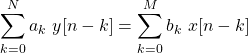
Using this representation its clearly depicted that the sum of weighted, delayed input impulses, x[n - k], is equal to a sum of weighted, delayed response impulses, y[n - k].

Homogeneous Equation

Setting the first sum equal to zero, and replacing y by some homogeneous response y_h, its easy to specify an homogeneous equation:



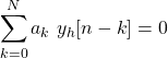
Whenever some particular y_p[n] satisfies the general equation, there exists some y_h[n], so that their sum y_p[n] + y_h[n] satisfies the homogeneous equation.

Notation used:

• y_p[n] : Particular solution
• y_h[n] : Homogeneous solution

Homogeneous Solution

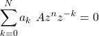
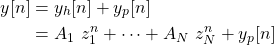
The homogeneous solution will be of the following exponential form:



which results into the following homogeneous equation:

The equation can be simplified to:



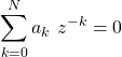
with the following N roots: z₁, z₂, ..., z_N, which give us the homogeneous solution:

Auxiliary Conditions

The homogeneous solution can be used in order to calculate the solution of the difference equation when combined with a particular solution:

In addition, N auxiliary conditions are also needed, such as the values of y for n_o = 0:



In Linear systems the initial conditions are mostly taken at 0. When speaking of Causal LTI systems, the initial rest is:

Explicit Recursive Solution

Assuming causality, when given:



its possible to calculate y[n_o]. Similarly the newly calculated value can then be used to calculate y[n_o + 1]. This procedure is therefore recursive.

As the initial, at rest solution is known from the auxiliary conditions, the solution is calculated from:

---

Block Diagram Representation

Mathematical representation always seems quite complex, and so block diagram representations have been developed.

Incorporate Delayed Impulses

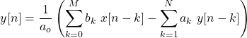
First of all, let's get into how the delayed impulses of the input and response can be visualized. Delayed impulses can be visualized using D squares. Interconnecting 1-sample delays with input and response lines result into the following representation:

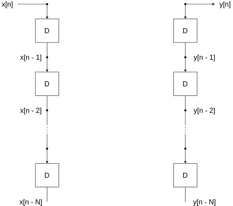
Incorporate Coefficients/Weight

In order to turn the delayed impulses into weighted delayed impulses, which is basically the same as including the coefficients of the LCCDE, we just have to multiply each x[n-k] and y[n-k] by those coefficients. Visually this can be interpreted as:

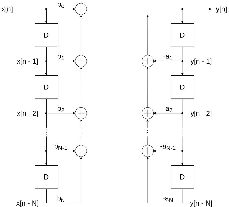
Sequence Sum Formation

Now that each part of the sums is known, let's also calculate those sums, which is as simple as:

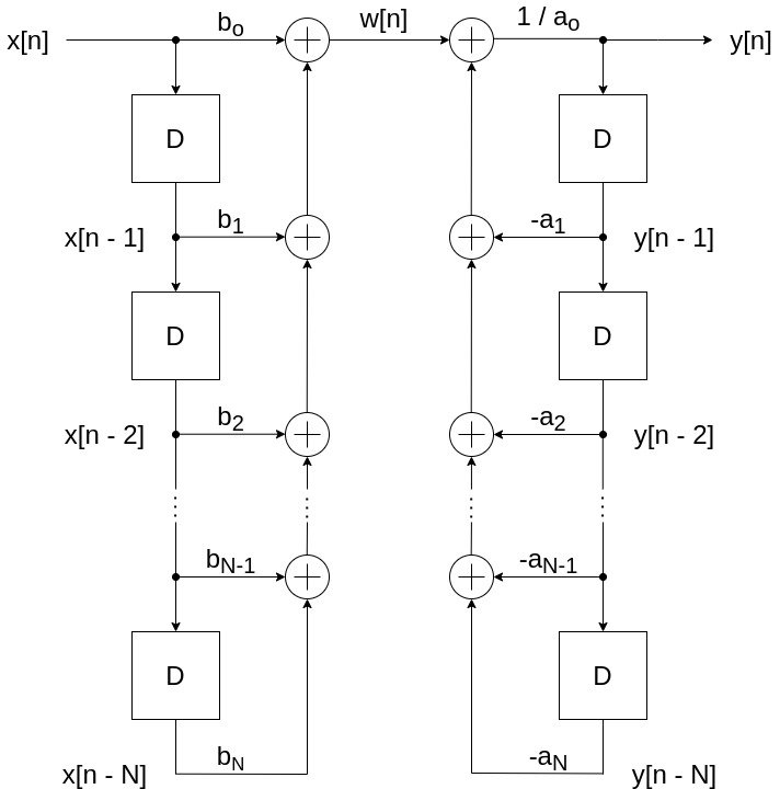
Direct Form I Implementation

If we also multiply by 1/a_o, we end up with a complete block diagram, known as the Direct Form I implementation:

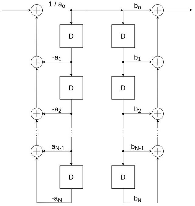
Due to the properties of LTI systems, its also possible to cascade these two segments in the opposite order. By also removing the x[n-k] and y[n-k] notations, as the coefficients suffice, we end up with the following interchanged block diagram:

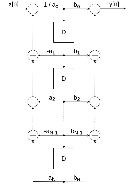
Direct Form II Implementation

Its also possible to make the block diagram even more compact by combining the two chains of delays. The resulting representation is known as the Direct Form II Implementation, which is visualized as follows:

---

RESOURCES:

References

1. Alan Oppenheim. RES.6-007 Signals and Systems. Spring 2011. Massachusetts Institute of Technology: MIT OpenCourseWare, License: Creative Commons BY-NC-SA.

Images

1. https://commons.wikimedia.org/wiki/File:From_Continuous_To_Discrete_Fourier_Transform.gif

Mathematical equations used in this article, where made using quicklatex.

---

Previous articles of the series

• Introduction → Signals, Systems
• Signal Basics → Signal Categorization, Basic Signal Types
• Signal Operations with Examples → Amplitude and Time Operations, Examples
• System Classification with Examples → System Classifications and Properties, Examples
• Sinusoidal and Complex Exponential Signals → Sinusoidal and Exponential Signals in Continuous and Discrete Time
• LTI System Response and Convolution → Linear System Interconnection (Cascade, Parallel, Feedback), Delayed Impulses, Convolution Sum and Integral
• LTI Convolution Properties → Commutative, Associative and Distributive Properties of LTI Convolution

---

Final words | Next up

And this is actually it for today's post!

Next time we will cover representation in Continuous-Time, which is done using Differential Equations...

See Ya!

Keep on drifting!