Mathematics - Signals And Systems - Signal Operations with Examples

about 3 years ago

Introduction

Hey it's a me again @drifter1!

I had exams and so I didn't have time for articles...but I'm back now and ready to rock 'n' roll!

Today we continue with my mathematics series about Signals and Systems in order to cover the Signal Operations with Examples.

So, without further ado, let's get straight into it!

Basic Signal Operations

Signals have two parameters that can be altered. Those are:

Amplitude
Time

A signal has a value called amplitude at each specific point in time, and each of those can be tweaked independently.

Amplitude Operations

The amplitude of a signal is the "value" that is has at a specific point in time. It basically shows us how far up or down from zero the signal's value is. The following operations can be applied on the amplitude of a signal:

Amplitude Scaling: scale the value of a signal by a factor
Signal Addition: add the amplitudes of two or more signals
Signal Subtraction: subtract the amplitudes of two or more signals
Signal Multiplication: multiply the amplitudes of two or more signals

Let's get into examples of each amplitude operations!

Amplitude Scaling

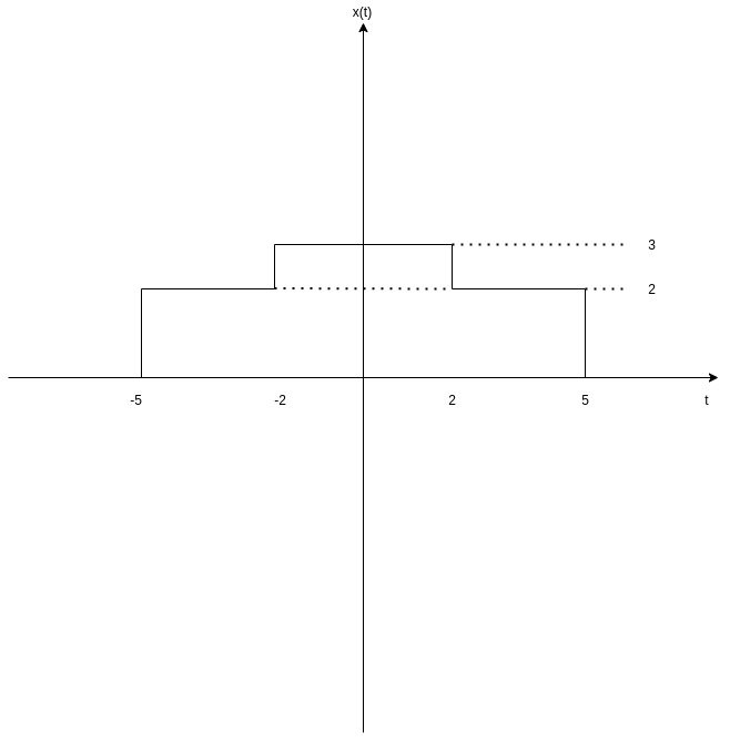
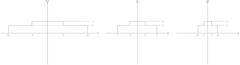
Suppose a continuous-time signal x(t) with the following graph over time:

[Custom Figure using draw.io]

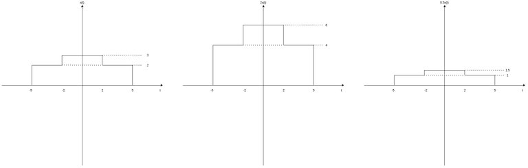
Scaling such a signal x(t) by some factor c results into another signal, c • x(t). The resulting signal is a scaled version of signal x(t), which means that the amplitude of x(t) is increased (or decreased) by a factor c, for each unit of time.

For example let's scale x(t) by c = 2 and c = 0.5. These two amplitude scaling operations give the following results:

[Custom Figure using draw.io]

It's easy to conclude that the signal 2 • x(t) has twice the amplitude of x(t) for each unit of time, whilst signal 0.5 • x(t) has half the amplitude. Let's also note that the whole operation was time-independent, and so the signal has "value" only at the points where it also had previously. Points in time where the amplitude was zero will stay zero after scaling with any factor c.

Addition

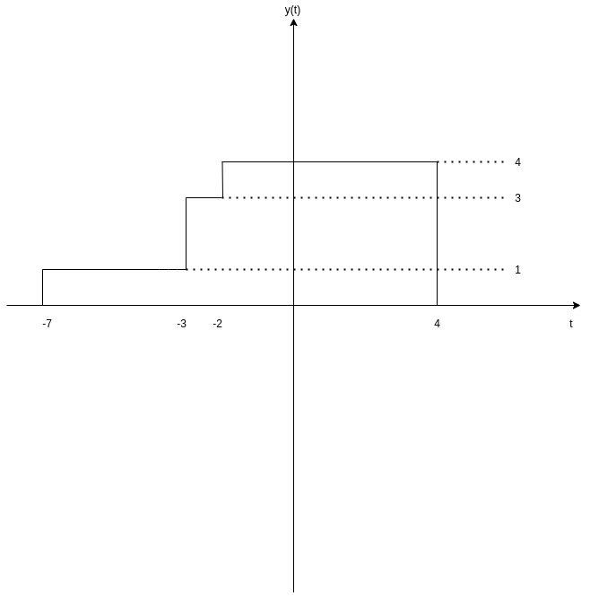
In addition to x(t), let's now also suppose a signal y(t) with the following graph:

[Custom Figure using draw.io]

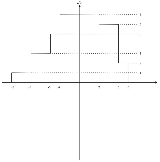
Adding the signals x(t) and y(t) results into a new signal, z(t) = x(t) + y(t). For each unit of time, this new signal has an amplitude that is equal to the addition of the corresponding ampltitudes of these two signals.

More specifically:

t < -7 → z(t) = 0
-7 ≤ t ≤ -5 → z(t) = 0 + 1 = 1
-5 ≤ t ≤ -3 → z(t) = 2 + 1 = 3
-3 ≤ t ≤ -2 → z(t) = 2 + 3 = 5
-2 ≤ t ≤ 2 → z(t) = 3 + 4 = 7
2 ≤ t ≤ 4 → z(t) = 2 + 4 = 6
4 ≤ t ≤ 5 → z(t) = 2 + 0 = 2
t > 5 → z(t) = 0

The graph of signal z(t) = x(t) + y(t) is:

[Custom Figure using draw.io]

Subtraction

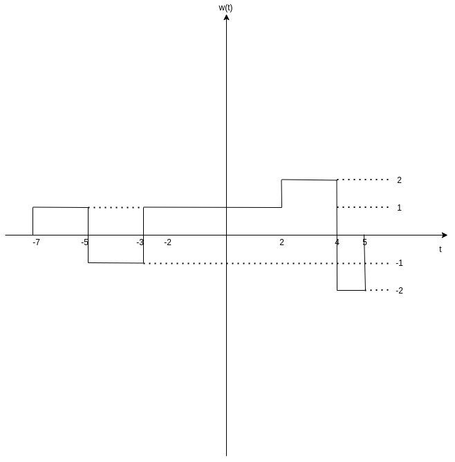
Subtracting signal x(t) from y(t) will result into a new signal w(t) = y(t) - x(t) where the amplitude of y(t) is "decreased" by the amplitude of x(t) for each unit of time.

Thus, we have:

t < -7 → w(t) = 0
-7 ≤ t ≤ -5 → w(t) = 1 - 0 = 1
-5 ≤ t ≤ -3 → w(t) = 1 - 2 = -1
-3 ≤ t ≤ -2 → w(t) = 3 - 2 = 1
-2 ≤ t ≤ 2 → w(t) = 4 - 3 = 1
2 ≤ t ≤ 4 → w(t) = 4 - 2 = 2
4 ≤ t ≤ 5 → w(t) = 0 - 2 = -2
t > 5 → w(t) = 0

The graph of signal w(t) = y(t) - x(t) is:

[Custom Figure using draw.io]

Let's also note that subtracting y(t) from x(t) would result into a different signal, let's call it v(t), which is basically -w(t).

So, the signal v(t) is an inverted version of signal w(t) along the time-axis:

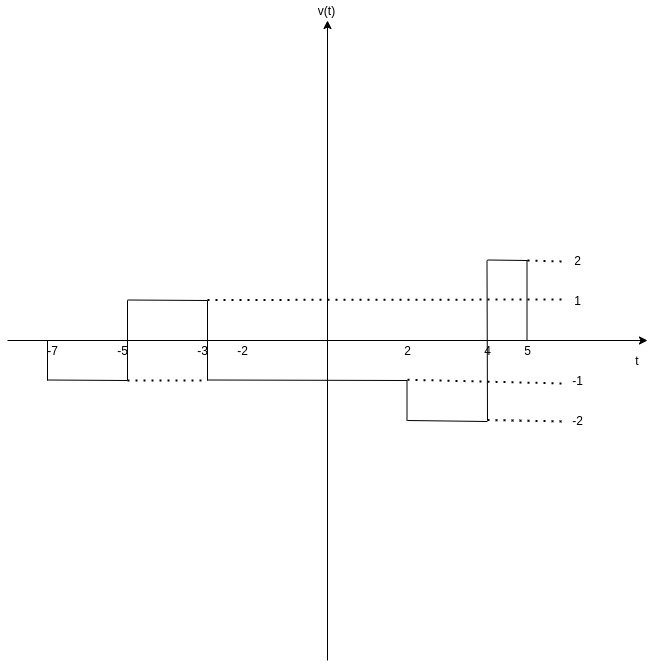
[Custom Figure using draw.io]

Multiplication

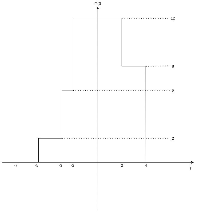
Multipliying the signals x(t) and y(t) results into a new signal m(t) = x(t) × y(t), with an ampltiude equal to the multiplication of the amplitude of the two signals for each unit of time.

In other words, we have:

t < -7 → m(t) = 0
-7 ≤ t ≤ -5 → m(t) = 0 × 1 = 0
-5 ≤ t ≤ -3 → m(t) = 2 × 1 = 2
-3 ≤ t ≤ -2 → m(t) = 2 × 3 = 6
-2 ≤ t ≤ 2 → m(t) = 3 × 4 = 12
2 ≤ t ≤ 4 → m(t) = 2 × 4 = 8
4 ≤ t ≤ 5 → m(t) = 2 × 0 = 0
t > 5 → m(t) = 0

Therefore, the graph of m(t) = x(t) × y(t) is the following:

[Custom Figure using draw.io]

Time Operations

In addition to amplitude, it's also possible to perform specific time operations.

Those are:

Time Shifting: negative or positive shifitng of a signal
Time Scaling: compression or expansion of a signal
Time Reversal: reversal of a signal

Let's get into examples of each time operations!

Time Shifting

The time-shifted version of a signal x(t) is denoted x(t &pm; t₀), where a positive t₀ value results into an negative shift, and vise versa.

Negative shifting (t + t₀) results into time delaying, whilst positive shifting (t - t₀) results into time advancing.

Let's consider the signal x(t) of the previous examples and shift it by 2 and -2, in order to understand the difference better.

The graphs of x(t - 2) and x(t + 2) are the following:

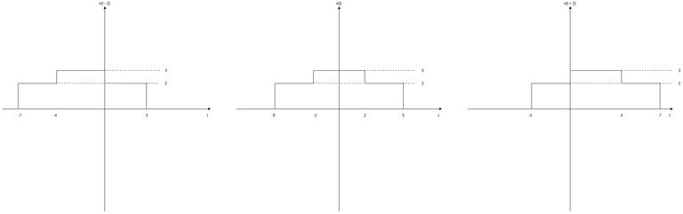
[Custom Figure using draw.io]

Its easy to conclude that negative shifting results in x(t) starting at -7 instead of -5, advancing the signal through time by 2 time units. On the other hand, positive shifting results in x(t) starting at -3 instead of -5, delaying the signal for 2 time units.

Time Scaling

Time scaling can be used in order to compress or expand a signal through time. A signal x(t) can be scaled through time by positive c, resulting into a signal x(c • t).

|c| > 1 → signal compression
|c| < 1 → signal expansion

Let's scale the signal x(t) of the previous examples by 2 and ½.

The graphs of x(2t) and x(t/2) are:

[Custom Figure using draw.io]

Its easy to notice that x(t/2) scales the duration of x(t) by 2 (-10 → 10 instead of -5 → 5), whilst x(2t) (de)scales the duration of x(t) by ½ (-2.5 → 2.5 instead of -5 → 5).

So, c = ½ < 1 truly resulted in signal expansion, whilst c = 2 > 1 truly resulted in signal compression.

Time Reversal

Lastly, there is also time reversal. Through time reversal its possible to "flip" the signal along the amplitude-axis (x-axis).

The signal x(t) is symmetrical and so x(t) = x(-t), where x(-t) is the time-reversed signal. So, let's use signal y(t) for this example. As we already said, y(-t) is basically y(t) but flipped along the x-axis.

Thus, the graph of y(-t) is simply:

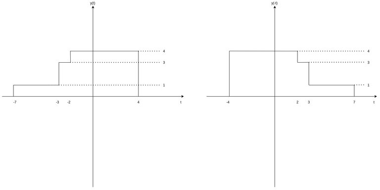
[Custom Figure using draw.io]