Mathematics - Signals And Systems - Exercises on System Representation using Differential Equations
![]()
[Image1]
Introduction
Hey it's a me again @drifter1!
Today we continue with my mathematics series about Signals and Systems in order to cover Exercises on System Representation using Differential Equations.
So, without further ado, let's dive straight into it!
Differential Equation Representation
Let's quickly recap how continuous-time LTI systems are represented.
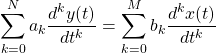
Such systems can be represented using linear constant-coefficient differential equations (LCCDE), which are of the form:
This representation can lead us to very useful Block Diagram Representations, such as the Direct Form I and II implementations.
In the examples that follow we will convert from one to the other, to understand those representations better.
Equation to Block Diagram [Based on P6.6 from Ref1]
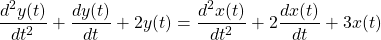
Let's first consider a LTI system that is represented by the following differential equation:
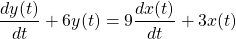
Let's draw the Direct Form I and II realizations of this system.
Solution
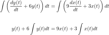
The diagram for continous-time systems contains integrator blocks, and so the first thing that one should do is integrate both sides of the given differential equation.
This leads us to the following:
Solving for y(t) leads to:
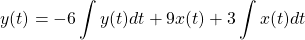
which can be easily turned into the Direct Form I implementation.
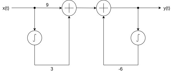
Now for the Direct Form II implementation.
First of all, the system is linear and time-invariant and so the two "sub-systems" can be easily interchanged as follows:
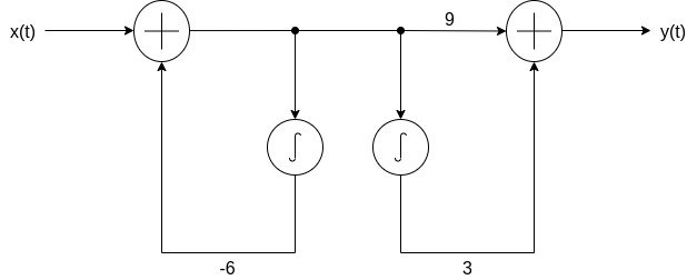
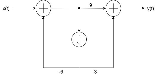
Combining the two integrators gives us the Direct Form II implementation:
Block Diagram to Equation [Based on P6.8 from Ref1]
Let's now do the opposite.
Consider the following Direct Form I Block Diagram that represents an LTI system:
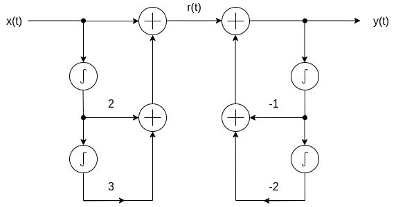
Let's find the differential equation representation for this system.
Solution
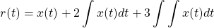
Let's first find the equation that describes the intermediate signal r(t).
Two integrations of x(t) are made and so:
Differentatiating twice yields the following result:
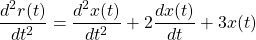
which shows us how x(t) and r(t) are related.
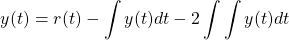
Now for the second "block". Relating y(t) and r(t) is as simple as:
Differentiating twice in order to get the second derivative of r(t) (and y(t) at the same time), and also solving for this derivative, gives us:
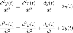
Equating these two relations, gives us the final answer that equates x(t) and y(t), which is:
This final representation can also be taken by using the "theory" block diagram as an example, but its easier to make mistakes that way. That's why I chose to insert an intermediate signal. Furthermore, this whole process is more convenient, easier to remember, and more applicable to any situation (and so even on non-standard forms of block diagrams).
RESOURCES:
References
Images
Mathematical equations used in this article were made using quicklatex.
Block diagrams and other visualizations were made using draw.io
Previous articles of the series
Basics
- Introduction → Signals, Systems
- Signal Basics → Signal Categorization, Basic Signal Types
- Signal Operations with Examples → Amplitude and Time Operations, Examples
- System Classification with Examples → System Classifications and Properties, Examples
- Sinusoidal and Complex Exponential Signals → Sinusoidal and Exponential Signals in Continuous and Discrete Time
LTI Systems and Convolution
- LTI System Response and Convolution → Linear System Interconnection (Cascade, Parallel, Feedback), Delayed Impulses, Convolution Sum and Integral
- LTI Convolution Properties → Commutative, Associative and Distributive Properties of LTI Convolution
- System Representation in Discrete-Time using Difference Equations → Linear Constant-Coefficient Difference Equations, Block Diagram Representation (Direct Form I and II)
- System Representation in Continuous-Time using Differential Equations → Linear Constant-Coefficient Differential Equations, Block Diagram Representation (Direct Form I and II)
- Exercises on LTI System Properties → Superposition, Impulse Response and System Classification Examples
- Exercise on Convolution → Discrete-Time Convolution Example with the help of visualizations
- Exercises on System Representation using Difference Equations → Simple Block Diagram to LCCDE Example, Direct Form I, II and LCCDE Example
Fourier Series and Transform
- Continuous-Time Periodic Signals & Fourier Series → Input Decomposition, Fourier Series, Analysis and Synthesis
- Continuous-Time Aperiodic Signals & Fourier Transform → Aperiodic Signals, Envelope Representation, Fourier and Inverse Fourier Transforms, Fourier Transform for Periodic Signals
- Continuous-Time Fourier Transform Properties → Linearity, Time-Shifting (Translation), Conjugate Symmetry, Time and Frequency Scaling, Duality, Differentiation and Integration, Parseval's Relation, Convolution and Multiplication Properties
- Discrete-Time Fourier Series & Transform → Getting into Discrete-Time, Fourier Series and Transform, Synthesis and Analysis Equations
- Discrete-Time Fourier Transform Properties → Differences with Continuous-Time, Periodicity, Linearity, Time and Frequency Shifting, Conjugate Summetry, Differencing and Accumulation, Time Reversal and Expansion, Differentation in Frequency, Convolution and Multiplication, Dualities
Final words | Next up
And this is actually it for today's post!
Next time we will start getting into exercises on the Fourier Series and/or Transform!
See Ya!
Keep on drifting!