Mathematics - Signals And Systems - Discrete-Time Sampling

almost 3 years ago

Introduction

Hey it's a me again @drifter1!

Today we continue with my mathematics series about Signals and Systems in order to cover Discrete-Time Sampling.

So, without further ado, let's dive straight into it!

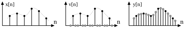
Getting into Discrete-Time Sampling

Until now, we used sampling as a way of processing continuous-time signals using discrete-time systems. But, sampling can also be applied to discrete-time signals, which in turn gives us the concept of discrete-time sampling (or Frequency Domain Sampling). The procedure is also quite similar to the one we used for continuous-time signals, in the sense that the discrete-time sequence is again multiplied by an periodic impulse train. With a period of N, this impulse train, might be used to retain every Nth sample of the original sequence, whilst the rest stays at zero. Of course, the same constraints of bandwidth also apply for discrete-time sampling, and so the original sequence can be recovered under the constraints of the sampling theorem. Furthermore, interpolation can again be implemented using an ideal low-pass filter.

Downsampling (or Decimation)

We can easily conclude that discrete-time sampling is quite similar to continuous-time sampling, so where is the difference? Well, discrete-time sampling is more of a downsampling or decimation procedure. After sampling the sequence, the newly obtained sequence has no practical reason to retain the zero values. Its explicitly used for retaining only every Nth sample, whilst sampling continuous-time signals is more of a way to approximate it.

Let's think about the special case where a continuous-time signal is sampled twice, in two steps. The second sampling that happens on the discrete-time representation (in the frequency domain) of course has to use a lower sampling rate then the one that was used originally. This basically means that sampling directly using this lower sampling rate would give the same signal, but in one step.

As we already mentioned in previous parts of the series, the sampling rate can have a quite important effect on the outcome of sampling. If the signal is periodic, a lower sampling rate (and so a decimation or downsampling) might still allow reconstruction, but in other cases it might be impossible to recover the original signal:

[Image 2]

Upsampling

The attempt of reconstructing the original sequence can be refered to as upsampling. This process can be split into 2 stages:

The N - 1 zero values that were removed while sampling are re-inserted between the sample points.
Interpolation is applied with a low-pass filter to re-construct the original sequence.

[Image 3]

Downsampling and upsampling can be used in lots of practical applications. As we already saw previously, one of them is sampling rate conversion. Incompatible systems can be made compatible by introducing such a sampling conversion layer.

RESOURCES:

References

Alan Oppenheim. RES.6-007 Signals and Systems. Spring 2011. Massachusetts Institute of Technology: MIT OpenCourseWare, License: Creative Commons BY-NC-SA.

Images

Mathematical equations used in this article were made using quicklatex.

Block diagrams and other visualizations were made using draw.io and GeoGebra

Previous articles of the series

Basics

Introduction → Signals, Systems
Signal Basics → Signal Categorization, Basic Signal Types
Signal Operations with Examples → Amplitude and Time Operations, Examples
System Classification with Examples → System Classifications and Properties, Examples
Sinusoidal and Complex Exponential Signals → Sinusoidal and Exponential Signals in Continuous and Discrete Time

LTI Systems and Convolution

LTI System Response and Convolution → Linear System Interconnection (Cascade, Parallel, Feedback), Delayed Impulses, Convolution Sum and Integral
LTI Convolution Properties → Commutative, Associative and Distributive Properties of LTI Convolution
System Representation in Discrete-Time using Difference Equations → Linear Constant-Coefficient Difference Equations, Block Diagram Representation (Direct Form I and II)
System Representation in Continuous-Time using Differential Equations → Linear Constant-Coefficient Differential Equations, Block Diagram Representation (Direct Form I and II)
Exercises on LTI System Properties → Superposition, Impulse Response and System Classification Examples
Exercise on Convolution → Discrete-Time Convolution Example with the help of visualizations
Exercises on System Representation using Difference Equations → Simple Block Diagram to LCCDE Example, Direct Form I, II and LCCDE Example
Exercises on System Representation using Differential Equations → Equation to Block Diagram Example, Direct Form I to Equation Example

Fourier Series and Transform

Continuous-Time Periodic Signals & Fourier Series → Input Decomposition, Fourier Series, Analysis and Synthesis
Continuous-Time Aperiodic Signals & Fourier Transform → Aperiodic Signals, Envelope Representation, Fourier and Inverse Fourier Transforms, Fourier Transform for Periodic Signals
Continuous-Time Fourier Transform Properties → Linearity, Time-Shifting (Translation), Conjugate Symmetry, Time and Frequency Scaling, Duality, Differentiation and Integration, Parseval's Relation, Convolution and Multiplication Properties
Discrete-Time Fourier Series & Transform → Getting into Discrete-Time, Fourier Series and Transform, Synthesis and Analysis Equations
Discrete-Time Fourier Transform Properties → Differences with Continuous-Time, Periodicity, Linearity, Time and Frequency Shifting, Conjugate Summetry, Differencing and Accumulation, Time Reversal and Expansion, Differentation in Frequency, Convolution and Multiplication, Dualities
Exercises on Continuous-Time Fourier Series → Fourier Series Coefficients Calculation from Signal Equation, Signal Graph
Exercises on Continuous-Time Fourier Transform → Fourier Transform from Signal Graph and Equation, Output of LTI System
Exercises on Discrete-Time Fourier Series and Transform → Fourier Series Coefficient, Fourier Transform Calculation and LTI System Output

Filtering, Sampling, Modulation, Interpolation

Filtering → Convolution Property, Ideal Filters, Series R-C Circuit and Moving Average Filter Approximations
Continuous-Time Modulation → Getting into Modulation, AM and FM, Demodulation
Discrete-Time Modulation → Applications, Carriers, Modulation/Demodulation, Time-Division Multiplexing
Sampling → Sampling Theorem, Sampling, Reconstruction and Aliasing
Interpolation → Reconstruction Procedure, Interpolation (Band-limited, Zero-order hold, First-order hold)
Processing Continuous-Time Signals as Discrete-Time Signals → C/D and D/C Conversion, Discrete-Time Processing