Generalized power law model of flow behavior at wellbore conditions while drilling
Greetings friends of the scientific and academic community of StemSocial and in general to all communities and users who make life within the platform in relation to STEM content.
In this opportunity I want to explain through this post the Generalized Power Law in which some equations involved in the flow behavior that is governed by the Power Law model will be explained, it is important to mention that it relates some graphs that simulate some of the equations governing the power law model.
Taking into consideration that the last topics discussed are intended to socialize with the whole community the importance of rheology within the well drilling activities, it is important that I can tell you that relating the behavior of drilling mud with the applications that have the flow equations to the well conditions during the drilling process is of utmost importance as it is a way to apply engineering to the actual conditions of drilling a particular petroleum well.
Introduction
It is necessary to explain the flow behavior through the consistency curves, especially taking into account that the consistency curves of most drilling fluids are intermediate between Bingham plastic fluids and ideal pseudoplastic fluid flow models, it is convenient to study the flow behavior of drilling fluids under a new approach, for this particular case and through the disclosure of this article is proposed as a new approach to study this stage of transition from these flow models to the generalized power law model.
It is important to demonstrate in this article, the difference between the consistency curves referring to shear stress versus strain rate of drilling fluids when subjected to low stress values, do not present a linear behavior as those of the power law model.
From the above I can say that having to study drilling fluids under the power law model represents a necessity in order to understand the nonlinearity in the consistency curves expressed by some drilling fluids.
Leaving a little of the power law flow model I also want to extend and treat in this article all the applications of the flow equations when they are adjusted to the well conditions while drilling, that is why it is necessary to ask:
Why do these equations have to be adjusted to the well conditions?
The equations used in the oil industry and in drilling to model the flow behavior of the drilling fluid are mainly based on the drilling mud temperature remaining constant throughout the entire circulation system, another condition on which these equations were structured is that the fluid properties are not thixotropic.
These ideal conditions mentioned above do not exist in the well while drilling, since it is impossible for the drilling mud to maintain a constant temperature during the entire cycle performed in its journey from the time it is driven by the mud pumps from the active tanks to the bottom of the well, the other is that drilling fluids must have that thixotropic characteristic to keep the cuttings in suspension when the pumps are paid.
That is why it is necessary that both conditions, constant temperature and thixotropy can be satisfied, as long as the rheological parameters can be determined under the flow conditions at that moment in some point of interest in the well. All these adversities and other conditions make attractive the study of the application of the equations that model the flow behavior of drilling mud to well conditions, which will be addressed in this article.
As third and last point to be explained, we have the flow conditions in the well, this topic is of great relevance if we take into account that the drilling mud will circulate through various spaces and all different in its path, when it leaves the active tank is transported by the pressure that prints the mud pump through a pipe, passing through the stand pipe until it reaches the drill pipe, it is there where it maintains a turbulent flow, but after it leaves the drill bit, it returns through the annular space (space between the hole and the drill pipe) until it reaches the active tanks again, the type of flow in the annular space is laminar.
Throughout this journey we can see the changes of regimes that the drilling mud has, everything is due to the actual conditions of the well, consequently to the diameters of pipe, well diameter, temperature at the bottom, among others. Under this point I will explain an exhaustive analysis of the well conditions that influence to have a particular flow regime.
Generalized Power Law
As I mentioned in the introduction, the consistency curves of most drilling fluids are intermediate between ideal Bingham plastic flow models and ideal pseudoplastic fluids. This is where the generalized power law comes into play, since this flow model extends the behavior of some drilling fluids, which are mostly dispersed fluids.
The nonlinear behavior in the logarithmic consistency curves show that n and k are not constant with the shear rate, that is to say that there is no proportion between the shear stress and the strain rate, there where it is evidenced a behavior different from the power law (linear behavior), so the traditional equation that describes the power law behavior can not be used and applied to determine the flow behavior of drilling fluids inside the drill pipe.
When it is required to model the nonlinear behavior of certain drilling fluids to power law, we see how certain characters gave certain model proposals such as the generalized power law model. It was Metzner and Reed developed the generalized power law to solve this difficulty.
Initially we could say that their work was based on the work initially developed by Rabinowitsch and Mooney, who showed that for laminar flow of any fluid, where shear stress represents only a function of the strain rate, the flow characteristics are completely defined by the ratio of the shear stress in the pipe walls to the strain rate to the strain rate in the pipe wall itself. We could say then that this was the main idea for the work initiated by Rabinowitsch and Mooney, however Metzner and Reed had to fix the equation proposed by Rabinowitsch and Mooney under the following structure:

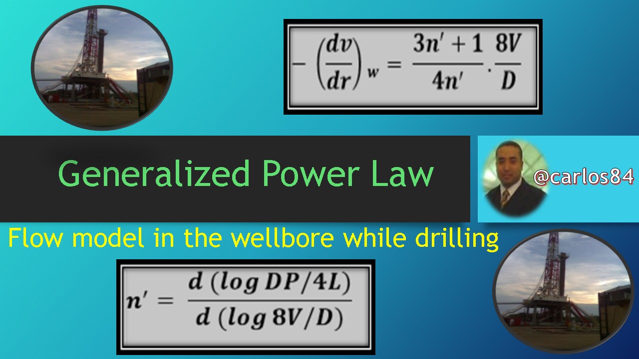
From this equation we can say that the term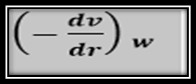 is the rate of deformation in the walls and that n' can be calculated as follows:
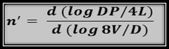
Where n' is numerically equal to n, y
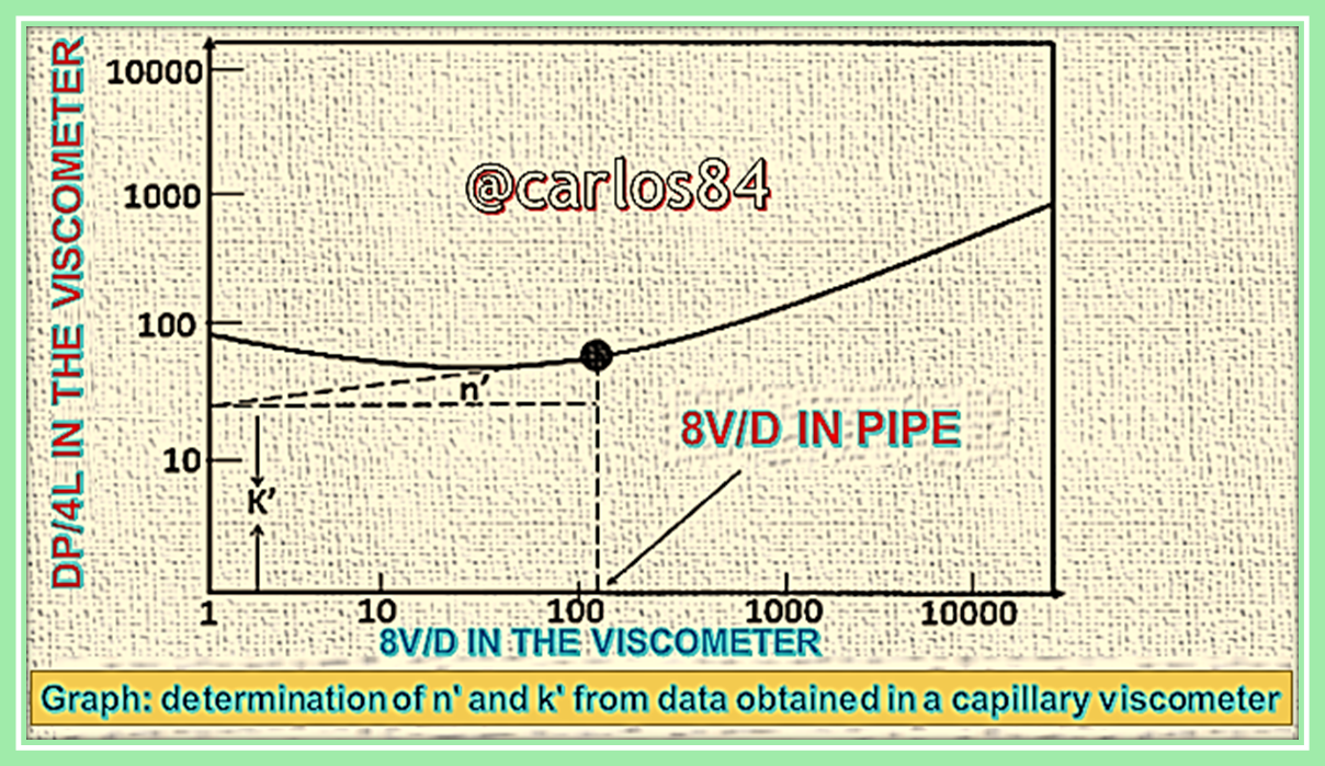
The advantage of employing the Power Law equation proposed by Rabinowitsch and Mooney is that compared to the flow model equation for pseudoplastic fluids is that the flow equation for pseudoplastic fluids is already integrated, and therefore, it is not a consequence of whether n or k are constant or not. Parameters such as n and k can be obtained from plots of the logarithm of DP/4L vs. 8V/D. When the curve is nonlinear, n' and k' are obtained from the tangent to the curve at the point of interest, as shown in the figure below:
The exact determination of the values of n' and k' from rotary viscometer data is more complicated to obtain, that is why alternative methods arise as the one proposed by Savins, who described a method based on the ratio of k' in the viscometer, although in actual practice more difficulties have been encountered to get the values of n and k, instead of presenting difficulty to get n' and k', then it can be said that to calculate the n and k should calculate these values at the rate of deformation to the current conditions that present the well while drilling.
It becomes necessary to perform a trial and error procedure, better known to engineers as the iteration method, the procedure consists of calculating n and k but in the appropriate velocity range on the multirotational viscometer.
As a verification method, the rate of deformation in the drill pipe walls can be calculated with the equation proposed by Metzner and Reed of the generalized power law, and if found to be considerably contrary to the rate at which n and k were evaluated, they have to be reevaluated and the pressure drop recalculated, that is how the trial and error method would be applied in this process.
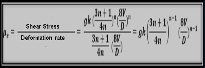
The effective viscosity of the drilling mud in the drill pipe is given by:
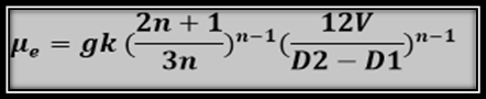
As I have been emphasizing in the development of the publication, it is necessary that all these equations are adopted and transformed to the real conditions of the well, then I must say that when the drilling mud circulates through the annular space, the rate of deformation in the walls is given by:

The effective viscosity transformed for the annular space is as follows:
Under what well conditions do the flow equations apply?
Up to this point a series of equations have been developed that model the flow behavior of drilling mud in the drill pipe and annulus, so those equations described in a rigorous manner are based primarily on:
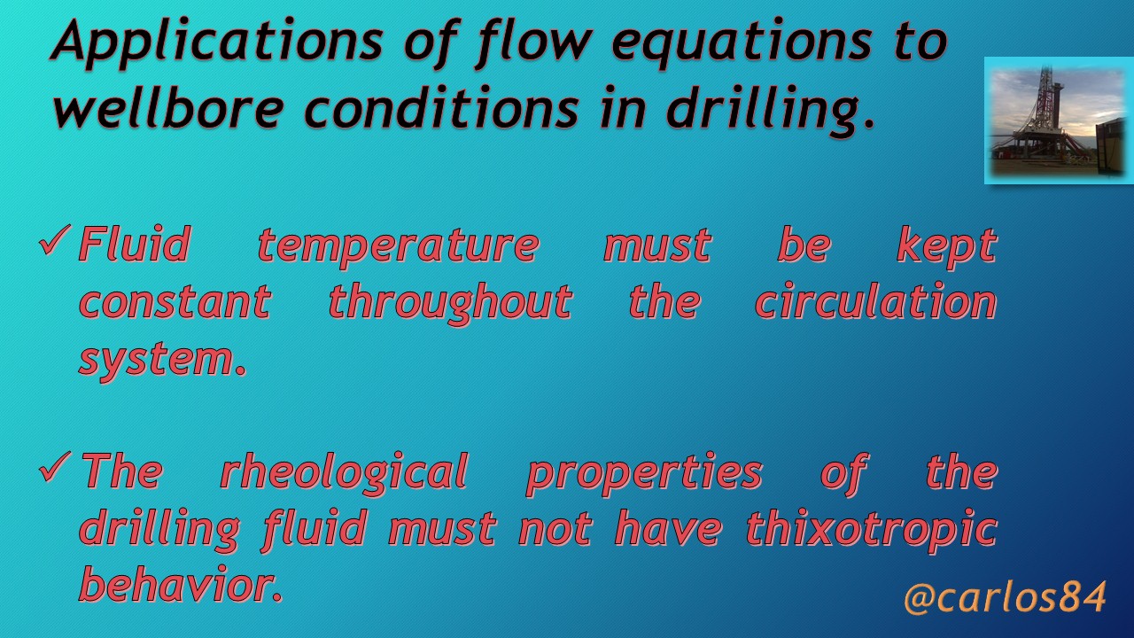
[1] The fluid temperature must be kept constant throughout the system.
[2] The rheological properties of the fluid must not have thixotropic behavior.
These two considerations or conditions are generally not present in the well being drilled, however both conditions can be overcome by determining the rheological parameters at the prevailing flow conditions at any point of interest in the well. However, there are difficulties, especially in being able to determine the flow conditions in which the drilling mud is found.
The temperature of the drilling mud is constantly changing and its precise value at a particular point in the circulation loop and at a particular time in the drilling cycle depends on several variables, also the strain rate undergoes drastic changes at different points in the loop and there is a considerable time lag before the shear rate reaches an approximate equilibrium.
In addition to these conditions, there are several unknown factors, such as the size of the annular space in flared sections of the hole, and another factor such as the rotation effect of the drill pipe.
Already taking into account these limitations, we can say that the flow pressures and velocities of drilling mud in the drilling of a well can never be evaluated at a predictive rate as perhaps they can be evaluated with the accuracy that can be achieved in a piping system in an industrial plant.
Due to these comparisons in the limitations to determine the flow pressures and transport velocities of drilling mud, a question arises, which will help us to understand the importance of being able to demonstrate the dependence of: the section of the flow circuit under consideration, the place where the research is being carried out, that is, whether in the laboratory of drilling fluids, or in the well being drilled.
The propitious question to be asked under this approach is:
Are these equations rigorous and the corresponding computer programs and in some cases justifiable in terms of time and expense given the inaccuracies that exist in the input data?
Everything is going to have a series of considerations, therefore it is going to depend on many factors, for example it is going to depend on the following factors:
Section of the flow circuit under consideration.
Purpose of the investigation and the place where the investigation is carried out (laboratory or drilling site), for this it is necessary to know the conditions in which the drilling mud flows in the well.
Flow conditions in the well
The flow conditions in which the drilling mud encounters as it is transported from the active tanks to the bottom of the wellbore will depend on the flow regime it has both in the drill pipe and in the annulus.
The flow in the drill pipe is generally turbulent and is only influenced by the viscous properties of the fluid to a minor degree. The effective shear rate at the pipe walls can be determined using capillary viscometry data. The dimensions of the pipe are known exactly, so that the pressure drop can be calculated almost exactly. The only inaccurate factor is the roughness of the drill pipe walls. The pressure drop in the drill pipe is about 20% to 45% of the pressure drop of a complete circulation system.
The velocity of the drilling fluid through the bit holes is extremely high, corresponding to a shear rate on the order of 100000 reciprocating seconds. The pressure drop across the bit holes can be accurately calculated because it depends on the discharge coefficient, which is essentially independent of the viscous properties of the mud. The pressure drop across the wick is about 50% to 75% of the pump discharge pressure.
Up to this point I have already described in a general way the conditions at which the drilling mud can be found inside the drill pipe until the moment it exits through the jets of the drill bit, it is time to make an analysis about the flow conditions at which the drilling mud can be found once it is in the annulus.
The flow of drilling mud in the annulus is normally laminar, and is therefore a function of the viscous properties of the mud. Shear rates are on the order of 50 to 150 reciprocating seconds. Although the pressure drop from bit to surface comprises only the range of 2% to 5% of the discharge pressure, it is therefore very important that pressures and flow rates in different sections of the annulus can be known when dealing with problems with hole cleaning, induced fracturing and hole erosion.
When the drilling mud is already in the annulus, unfortunately, accurate predictions of flow relationships are generally very difficult to predict because there are factors that generate uncertainty due to lack of knowledge.
One of the factors that generates this uncertainty is the diameter of the hole, since it is very difficult that the diameter of the hole is the same of the drill bit, for example if we drill with a 17-1/2 inches bit, not necessarily the diameter of the hole is 17-1/2 inches, since depending on the lithology of the rock and the flow velocity, the formation can be undermined, and make that there are sections with a diameter greater than 17-1/2 inches.
Even the actual diameter of the hole can be twice the nominal diameter, especially in sections of the well where the hole is widened, causing the lifting velocity to decrease four times its value.
The following figure depicts a typical hole enlargement in the section of the hole where shales are present:
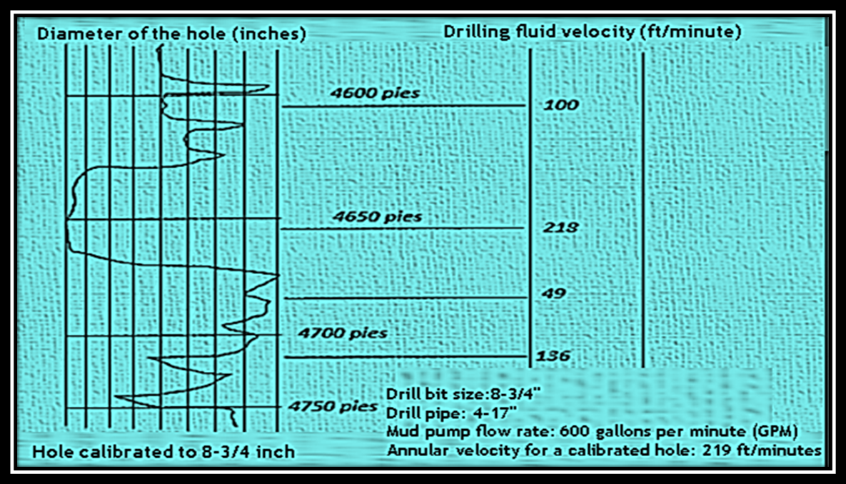
In the graph we can notice that a well is being drilled with an 8-3/4 inch diameter bit, where we can analyze a profile from 4600 feet to 4750 feet. We can see that at 4600 feet we have a velocity of 100 ft/minute, and when we reach the depth of 4650 feet the mud velocity increases due to the hole diameter approaching the nominal diameter of 8-3/4 inches, while when approaching 4700 feet it has a decrease in velocity as it falls into a widened section of the hole.
In conclusion, when you have a hole section where there is a widening in the diameter due to a shale zone, you have changes in the velocity profile of the drilling fluid transport in the annulus. The influence of drillstring rotation on the velocity profiles is also difficult to take into account. Equations for helical flow exist, but they were derived for drill strings rotating in a vertical hole, whereas in practice, the drillstring moves in a deviated hole in a disorderly manner.
Finally I can tell you on this point that there is no practical way to account for the influence of thixotropy on the viscosity of the drilling mud especially as it rises in the annulus.
Conclusions and final considerations
[1] The high shear rate in the drill pipe and bit jets reduces the structural component of the viscosity to a very low value: this condition makes the shear rates in the annulus much lower, however they are subject to change in any section of the annulus section, especially if we take into consideration the unknown or uncertainty about the actual hole diameter.
[2] Considering the low shear rates in the annulus, we can add other conditions to the variant in the uncertainty of the hole diameter, among these other variants are: drill collars diameter, drill pipe diameter, casing diameter and the degree of hole enlargement. These considerations lead me to think that assuming that the hole is not enlarged, the existence of a larger diameter by some component of the drill string will cause a reduction or enlargement of the annular space (space between the hole and the drill string).
[3] The viscosity of the drilling mud adjusts at each rate of deformation to which it is subjected, but it is important to consider that it takes considerable time to do so, and may never reach the equilibrium value, except in long sections of the hole where a constant diameter is maintained, or the fluid is in a cased hole section where there is no change in diameter. From my experience in drilling, my recommendation is that if you are drilling a hole with a drilling mud with some initial conditions, in which you want to restore its properties, especially the viscosity, circulate it at least two hours before starting the drilling of the subsequent hole.
In summary and as a final conclusion we have that the pressure drops in the drill string in the bit can be calculated exactly with the equations that have as a condition of laminar flow, while in the annular space are much more questionable such calculations, since there are several variables that suddenly change the character of fluid flow, such as fluid velocity, pressure drops among others.
However the pressure drops in the whole circuit can be calculated accurately because the pressure drops in the annulus are a small percentage of the total that the drilling mud can present in the whole cycle from its journey from the active tanks to reach the bottom of the hole, and return through the annulus until it reaches the active tanks again.
References
Observations
All the images and equations are of my authorship, they were elaborated using Microsoft Office 2010 tools.