[SPA-ENG] "Citizen Science" Project - Report - Part Six | Reporte - Sexta parte
Este es mi reporte de la sexta parte del proyecto de ciencia ciudadana. En la parte anterior, simulamos la señal de neutrinos. Para más detalles, pueden leer mi reporte o el de cualquiera de mis compañeros de proyecto en la etiqueta #citizenscience. En esta parte, vamos a ocuparnos de las incertidumbres inherentes al cálculo. Si quieren conocer más sobre este proyecto, pueden ingresar a este post de @lemouth, que es quien está liderando este experimento en Hive.
This is my report of the sixth episode of the citizen science project. In the previous part, we simulated the neutrino signal. For more details, you can read my report or that of any of my project partners under the tag #citizenscience. In this part, we are going to deal with the uncertainties inherent in the calculation. If you want to learn more about this project, you can go to this post by @lemouth, who is leading this experiment at Hive.
¿Por qué las incertidumbres? Bueno, porque ahora nos cuenta lemouth que el cálculo de la tasa de producción asociada a la señal anterior es un cálculo perturbativo. No tenía ni idea de qué es un cálculo perturbativo, pero la explicación de lemouth es muy clara. Voy a tratar de parafrasearla. El cálculo en cuestión es perturbativo porque se puede escribir como una serie infinita en la cual el primer término (leading-order calculation) es el dominante y luego viene una corrección secundaria (subleading) tras otra, hasta el infinito. Como no es posible tener en cuenta las infinitas correcciones, debemos cortar la serie infinita en algún punto, lo que da lugar a esa incertidumbre de la que hablábamos. Cuánto mayor sea la cantidad de correcciones que calculemos, menor será la incertidumbre. Lo que vamos a hacer en este episodio, entonces, es volver a calcular la señal, pero en este caso, estimando también la incertidumbre inherente al cálculo.
Why the uncertainties? Well, because lemouth now tells us that the calculation of the production rate associated with the above signal is a perturbative calculation. I had no idea what a perturbative calculation is, but lemouth's explanation is very clear. I will try to paraphrase it. The calculation in question is perturbative because it can be written as an infinite series in which the first term (leading-order calculation) is the dominant one and then comes one secondary correction (subleading) after another, to infinity. Since it is not possible to take into account the infinite corrections, we must cut the infinite series at some point, which gives rise to the uncertainty we were talking about. The greater the number of corrections we calculate, the smaller the uncertainty. What we are going to do in this episode, then, is to recalculate the signal, but in this case, also estimating the uncertainty inherent in the calculation.
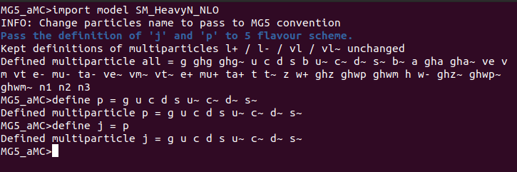
Para hacer este cálculo vamos a seguir usando las herramientas del episodio anterior: nuestro ya viejo conocido MG5aMC y el modelo heavyN. Una vez iniciado MG5aMC, importé el modelo y definí el contenido del protón.
To do this calculation we are going to continue using the tools from the previous episode: our old familiar MG5aMC and the heavyN model. Once MG5aMC was started, I imported the model and defined the proton content.
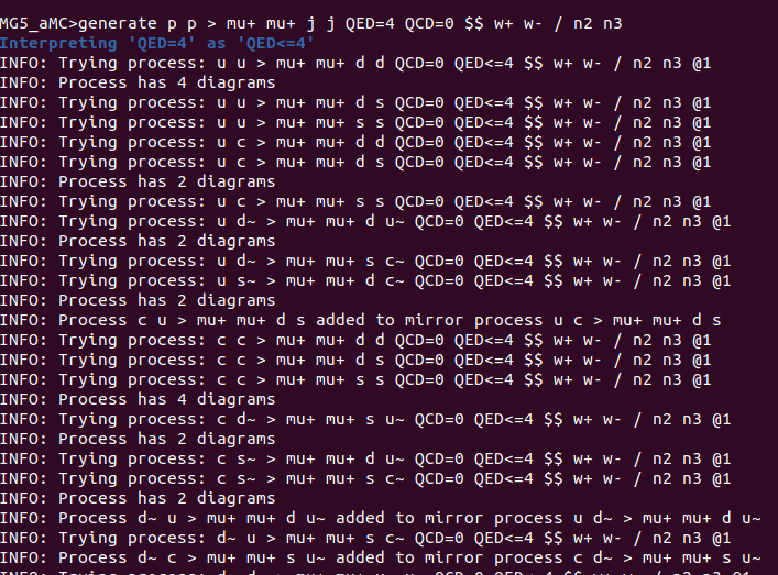
Luego, generé las colisiones:
Then, I generated the collisions:
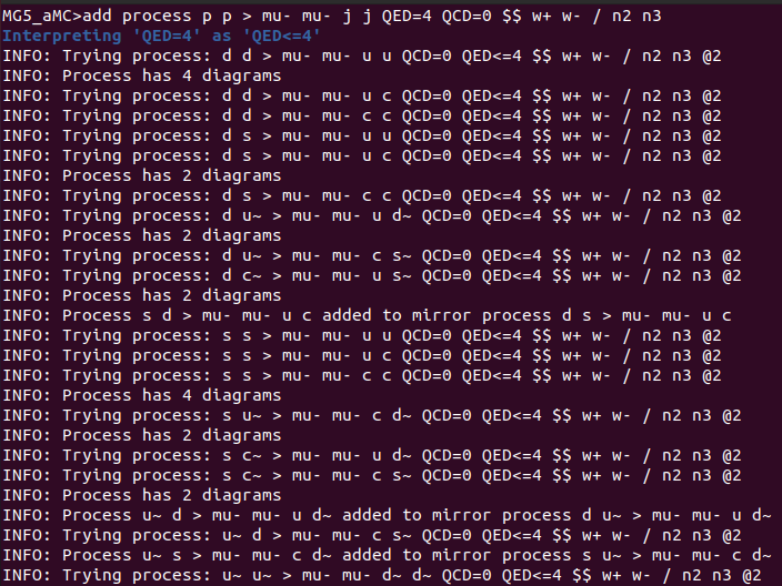
La agregué:
I added it:
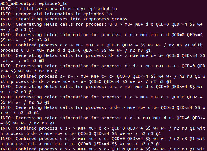
Y finalmente creé el directorio de trabajo:
And finally I created the working directory:
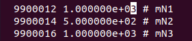
Hasta aquí nada nuevo. Ahora llegó el momento de hacer el cálculo otra vez pero estimando la incertidumbre, que es el objetivo principal de este episodio. Para ello, lancé primero el programa con la configuración por defecto y luego ajusté los parámetros del archivo del modelo de neutrinos para que se ajuste a un escenario en el que un neutrino pesado N interactúa con muones y antimuones. Primero ajusté la masa del neutrino pesado:
So far nothing new. Now it was time to do the calculation again but estimating the uncertainty, which is the main goal of this episode. To do this, I first launched the program with the default settings and then adjusted the parameters of the neutrino model file to fit a scenario in which a heavy neutrino N interacts with muons and anti-muons. I first adjusted the mass of the heavy neutrino:
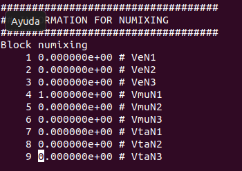
Y para terminar dejé activo solo el acoplamiento del neutrino pesado a los muones.
And finally I left active only the coupling of the heavy neutrino to the muons.
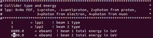
Luego, edité la run card. Para ello, primero seteé la energía de los haces de colisión en 6800 GeV, como corresponde al LHC Run 3.
Then, I edited the run card. To do this, I first set the energy of the collision beams to 6800 GeV, as corresponds to LHC Run 3.
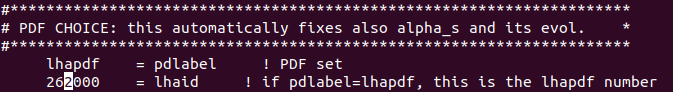
Elegí lhapdf:
I chose lhapdf:
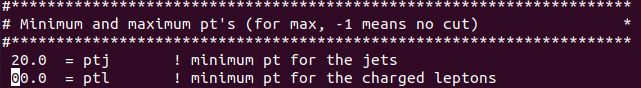
Y llevé el mínimo ptl a 0:
And I brought the minimum ptl to 0:
Y finalmente dejé que el software haga los cálculos.
And finally I let the software do the calculations.
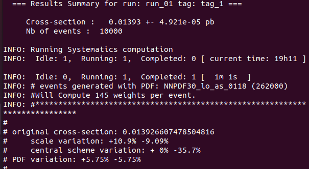
Los resultados son ligeramente diferentes a los de lemouth (en lugar de 0,0138, obtuve 0,01393 de cross-section).
Luego, modifiqué modifiqué los valores de la masa de este modo:
The results are slightly different from lemouth's (instead of 0.0138, I got 0.01393 cross-section).
Then, I modified the mass values in this way:

Y obtuve los siguientes resultados:
And I obtained the following results:
run_name | mass#9900012 | cross | scale variation | PDF variation
run_02 | 5.000000e+01 | 3.843400e-03 | +2.56% -2.67% | +5.87% -5.87%
run_03 | 2.500000e+02 | 1.626660e-02 | +6.39% -5.74% | +5.69% -5.69%
run_04 | 5.000000e+02 | 1.791950e-02 | +8.61% -7.42% | +5.69% -5.69%
run_05 | 1.000000e+03 | 1.390020e-02 | +10.9% -9.09% | +5.73% -5.73%
run_06 | 2.500000e+03 | 5.715200e-03 | +13.4% -10.8% | +5.89% -5.89%
run_07 | 5.000000e+03 | 1.999210e-03 | +15% -11.9% | +6.03% -6.03%
run_08 | 7.500000e+03 | 9.832500e-04 | +15.4% -12.2% | +6.11% -6.11%
run_09 | 1.000000e+04 | 5.719200e-04 | +15.6% -12.3% | +6.12% -6.12%
run_10 | 1.500000e+04 | 2.623280e-04 | +15.8% -12.4% | +6.13% -6.13%
run_11 | 2.000000e+04 | 1.501200e-04 | +15.7% -12.4% | + 6% - 6%
Que, con la incertidumbre total calculada, resultan en:
That, with the total uncertainty calculated, they result in:
run_name | mass#9900012 | cross | upper | lower
run_02 | 5.000000e+01 | 3.843400e-03 | 6.40% | 6.45%
run_03 | 2.500000e+02 | 1.626660e-02 | 8.56% | 8.08%
run_04 | 5.000000e+02 | 1.791950e-02 | 10.32% | 9.35%
run_05 | 1.000000e+03 | 1.390020e-02 | 12.31% | 10.75%
run_06 | 2.500000e+03 | 5.715200e-03 | 14.64% | 12.30%
run_07 | 5.000000e+03 | 1.999210e-03 | 16.17% | 13.34%
run_08 | 7.500000e+03 | 9.832500e-04 | 16.57% | 13.64%
run_09 | 1.000000e+04 | 5.719200e-04 | 16.76% | 13.74%
run_10 | 1.500000e+04 | 2.623280e-04 | 16.95% | 13.83%
run_11 | 2.000000e+04 | 1.501200e-04 | 16.81% | 13.78%
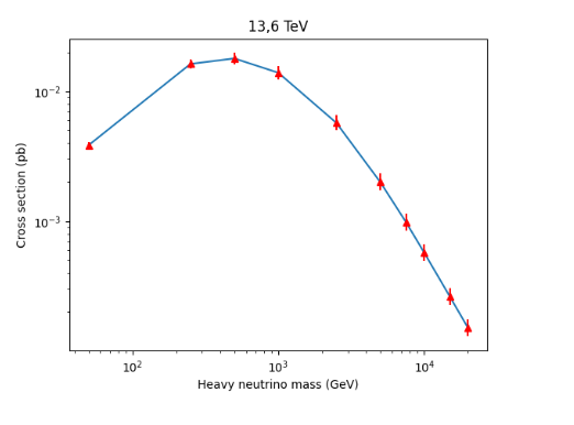
Para hacer el gráfico tuve que investigar un poco, porque no tengo muchos conocimientos de matplotlib. Como en el episodio anterior, usé un compilador online de Matplotlib. Calculé los porcentajes en una planilla de cálculo, porque no pude encontrar cómo hacerlo en matplotlib. El resultado es este (espero que esté bien…):
To make the graph I had to do some research, because I don't have much knowledge of matplotlib. As in the previous episode, I used an online matplotlib compiler. I calculated the percentages in a spreadsheet, because I couldn't find how to do it in matplotlib. The result is this (I hope it's ok...):
to do the plot, you can also try Rstudio (using R) they have a cloud version online

!1UP
Thank you very much! I will try Rstudio for the next one.
You have received a 1UP from @gwajnberg!
@stem-curator, @vyb-curator, @pob-curator, @neoxag-curator
And they will bring !PIZZA 🍕.
Learn more about our delegation service to earn daily rewards. Join the Cartel on Discord.
Congratulations for this report. Today was a great day, with two reports being delivered at once: yours and that of @travelingmercies. So two great readings for tonight for me, right before my departure for HiveFest in Amsterdam.
I wanted to keep the two reviews for the train trip, but I could not resist, and I finally decided to go through the reports immediately. I started with your report as you posted it first. I will probably handle that of @tralveingmercies tomorrow morning (as it is almost midnight here).
Your work is very good, and As usual, I have a few comments. These comments are however minor comments. Don't worry! The results look perfect.
Your paraphrasing is totally correct. You got very precisely the point!
Technically, we don’t generate ‘one collision’, but a sample of collisions giving rise to the same final state (the final state that we indicated: two leptons and two jets). However, each collision is different in the sense that the properties of the final-state particles (their energy, momentum, etc.) are different. Those differences reproduce the distributions expected from nature. The more likely configurations will appear more often, and the less likely ones less often.
Of course, this is true once we assume the underlying model of physics that we imported in the code, with the chosen set of parameters. If we change something there then the predictions will be different.
Although our results are different (this is normal, as we rely on a Monte Carlo integration method that depends on random numbers), they are numerically compatible (after accounting for the numerical error of about 1%, which is different from the theoretical uncertainties inherent to the calculation and that are of order 10%).
Note that the total uncertainties are relative uncertainties. Those should be percents. This should be added to the second table.
It looks very OK to me. Congratulations! It is a total success!
Thank you very much for the clarifications and corrections! I edited the part that talked about "one collision" and added the percentage symbols in the table. I'm glad the chart is correct! Matplotlib is giving me headaches because I don't quite know how to use it. is there any way to tell matlib directly the percentages for the error bars? Cheers!
The easiest would be to first computing the absolute errors in Python (by manipulating the list of central values and the list of errors, or in an easier way by manipulating twice a single list with everything in it), and then feeding Matplotlib with them. Including the calculation directly in matplotlib would allow you to avoid having to calculate them by yourself.
If you want, I can show you how to do it (but you will need to provide your code under a form I could copy paste it to modify it ;) ).
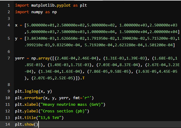
Thank you very much! If you have time, I would like to learn how to do it directly in the code. This is the code I used for the plot:
import matplotlib.pyplot as plt
import numpy as np
x = [5.000000e+01,2.500000e+02,5.000000e+02, 1.000000e+03,2.500000e+03,5.000000e+03,7.500000e+03,1.000000e+04, 1.500000e+04,2.000000e+04]
y = [3.843400e-03,1.626660e-02,1.791950e-02,1.390020e-02,5.715200e-03,1.999210e-03,9.832500e-04, 5.719200e-04,2.623280e-04,1.501200e-04]
yerr = np.array([(2.48E-04,2.46E-04), (1.31E-03,1.39E-03), (1.68E-03,1.85E-03), (1.49E-03,1.71E-03), (7.03E-04,8.37E-04), (2.67E-04,3.23E-04), (1.34E-04,1.63E-04), (7.86E-05,9.58E-05), (3.63E-05,4.45E-05), (2.07E-05,2.52E-05)]).Tplt.loglog(x, y)
plt.errorbar(x, y, yerr, fmt='r^')
plt.xlabel("Heavy neutrino mass (GeV)")
plt.ylabel("Cross section (pb)")
plt.title("13,6 TeV")
plt.show()
Let's assume you have an output vector with both y central value and relative errors:
Then you can obtain the absolute errors and central value as:Cheers!
Thanks a lot! I will try it. Cheers!
Thanks for your contribution to the STEMsocial community. Feel free to join us on discord to get to know the rest of us!
Please consider delegating to the @stemsocial account (85% of the curation rewards are returned).
Thanks for including @stemsocial as a beneficiary, which gives you stronger support.
Thanks so much for your support!