Physics 000 - Acceleration, Velocity & Displacement in One Dimension

over 2 years ago (Edited)

Introduction

This is the first in a series of posts covering physics. Why bother create a bunch of posts covering what many people here probably already know? The main reason for me to do this is because I typically create content before I need it in other content. So, I am creating this to reference later in other educational content.

Reference Frames
A discussion of physics should begin with an important but brief topic, which is reference frame, or frame of reference. For example if two people, Person A and Person B, are standing shoulder-to-shoulder but facing opposite directions, each person has a different frame of reference. Forward to Person A is reverse to Person B. Likewise left to one is right to the other. However, both share a commone reference for up and down, because they are both standing "upright". However, if one is flipped upside down in addition to facing the opposite direction of the other, they will no longer share a common reference for up. Up to one will be down to the other. We can also call each person's reference frame a local reference.

Position, Displacement & Distance
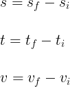
Position is expressed in meters. The difference between two positions is called the displacement. Displacement can be calculated as

$s=\Delta P=P_f-P_i$
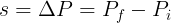
where
$\\s=displacement\\\Delta P=change\ in\ position\\P_i=initial\ position\\P_f=final\ position$

The terms displacement and distance are sometimes used interchangably, although they mean two different things. Displacement is a vector quantity, meaning it has both a magnitude and direction, while distance is a scalar quantity and can never be negative. For example, an object can be displaced 5m then displaced another -10m. The object's displacement from the starting point will be -5m and its distance from the starting point will be 5m. Its total distance traveled will be 15m.

Suppose an object's initial position is 0 meters and its final position is -1 meter, the displacement is -1m. Perhaps an object started out at 150 meters and ended up at 155 meters, the distance it traveled is 5m. Displacements can be negative because the sign indicates the direction, either forward or backward.

Velocity
Velocity is a change in position over a period of time, or expresed in terms of distance, a distance traveled over a period of time. Time is expressed in seconds. Therefore velocity can be written as

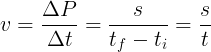
$v=\frac{\Delta P}{\Delta t}=\frac{s}{t_f-t_i}=\frac{s}{t}$
where
$\\v=velocity,\ in\ meters\ per\ second\\\Delta t=change\ in\ time\\t_i=initial\ time,\ in\ seconds\\t_f=final\ time,\ in\ seconds\\t=time,\ in\ seconds$

For example, if an object moved a distance of 5 meters over 2 seconds, its velocity was 2.5m/s. If an object took 10 seconds to move -1 meter its velocity was -0.1m/s. Both are shown below. Note that, as used above, t and delta t both express the same thing, a change in time. The initial and final time are specific instants in time. Unless otherwise noted, all changes in time in this post will be referred to as t. As with displacement, velocities may be negative due to the frame of reference being used.

$v=\frac{5m}{2s}=\frac{2.5m}{s}=2.5m/s\\\\\\v=\frac{-1m}{10s}=\frac{-0.1m}{s}=-0.1m/s$

Although some use the terms velocity and speed interchangably, they are not the same thing. Velocity is a vector quantity while speed is a scalar quantity. For example, suppose you are driving on the highway and get pulled over by a police officer, who asks you if you know how fast you were going. You respond with some number, probably whatever the speed limit is. Because your response only included speed, it is not velocity. If you would have responded with a speed and direction, such as "going north at 75mph", you would have specified a velocity.

Acceleration
Acceleration (a) is a change in velocity over a period of time, or expressed in terms of velocity, the velocity added to or subtracted from an existing velocity over a period of time. This post will only deal with constant acceleration, that is acceleration that does not change and is "all or none". Acceleration is given in meters-per-second per-second, or meters-per-second squared, and may be positive or negative.

Example Scenario

Unless otherwise noted, time will always be plotted along the x-axis of graphs, while a graph's y-value may be acceleration, velocity, or distance depending on the circumstance.

Accelerating an Object
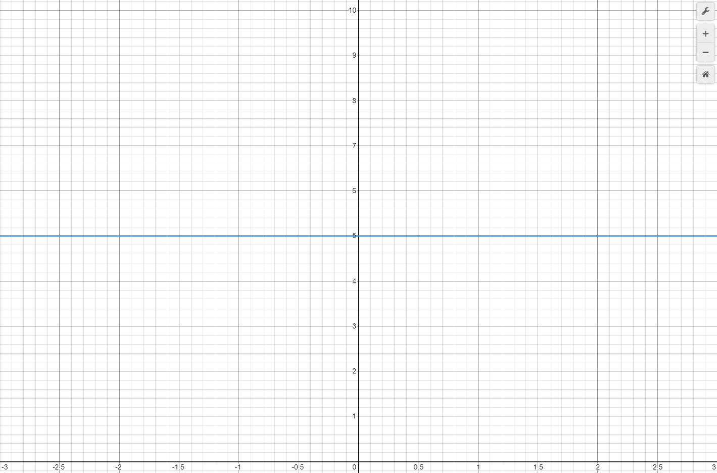
Suppose an object starts out with a velocity of 0m/s and is accelerated at 5m/s/s (meters per second, per second). This means for each second that passes, the object's velocity increases by 5m/s. At the end of the first second, its velocity will be 5m/s, by the end of the 2nd second it will be 10m/s, and by the third second the velocity will be 15m/s. The function describing a 5m/s/s constant acceleration is

$y=5$

Because this is constant acceleration, it is 5m/s at all times and does not increase or decrease, as shown by the horizontal blue line in Graph 1.

Graph 1 - Constant acceleration of 5m/s/s

Finding the Object's Velocity
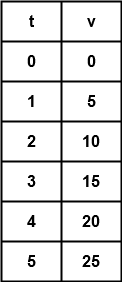
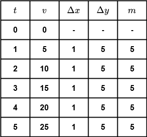
Visualizing the object's velocity using a graph is easy, we simply create a table listing the velocity at each second then plot the results on a graph. Table 1 lists the velocities for the first five seconds of acceleration, and Graph 2 shows the first three of these points.

Table 1 - Velocity versus time

Grap 2 - Velocity points for 5m/s/s acceleration

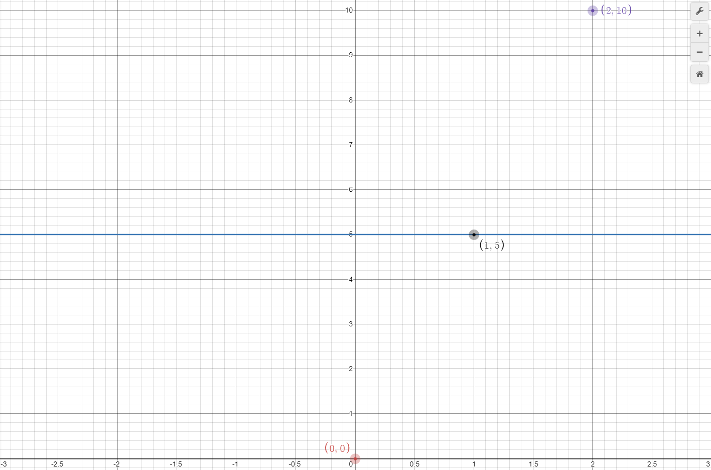
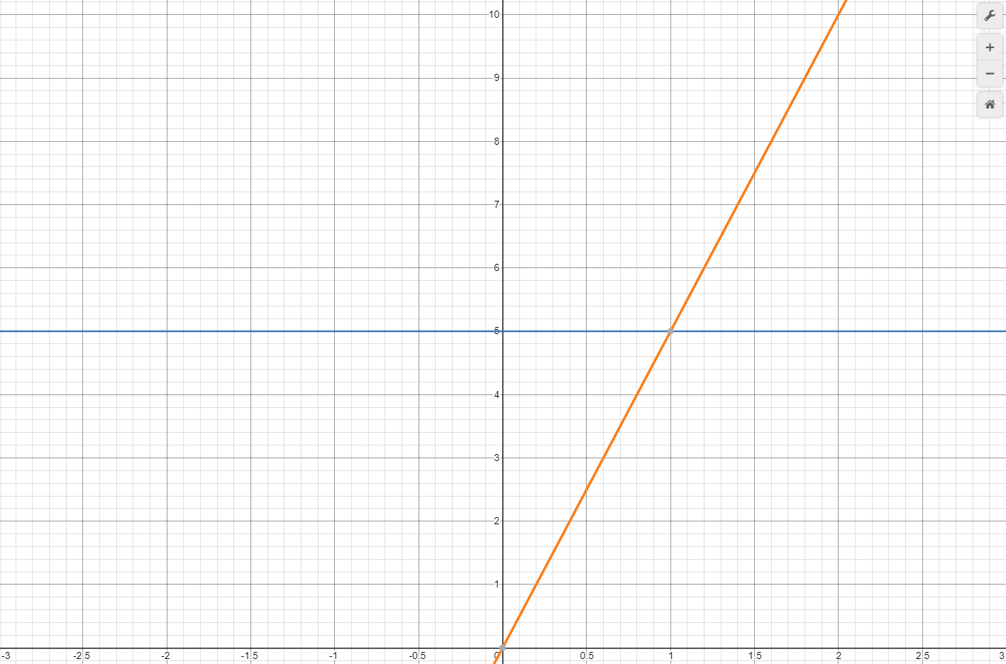
Merely plotting individual points on a graph usually does not give a good indication of the shape of a curve, so it is better to draw a lines connecting points. In the case of velocity, this is just a single line with some slope, as shown in orange on Graph 3.

Graph 3 - Velocity curve for 5m/s/s acceleration

Slopes
Slope of lines is another important topic which should be briefly covered, and expresses how much (magnitude and direction) the y-value of a function changes for each change in the function's x-value. The formula for slope is

$m=\frac{\Delta y}{\Delta x}=\frac{y_1-y_0}{x_1-x_0}$

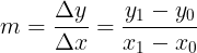
where

$\\m=slope\\\Delta x=change\ in\ x\\\Delta y=change\ in\ y\\(x_0,y_0)=coordinates\ of\ first\ point\\(x_1,y_1)=coordinates\ of\ second\ point$

For example, if the first point of a line is at (-3, 1) and the second point is at (4, 6), the line's slope would be approximately 0.7143.

$m=\frac{6-1}{4-^-3}=\frac{5}{7}\approx 0.7143$

Turning back to the velocity line for an acceleration of 5m/s/s and solving for the first two points

$m=\frac{5-0}{1-0}=\frac{5}{1}=5$

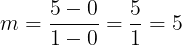
Table 2 shows the slopes for the remaining four points. It is evident the slope does not change, at least within the limits set by the calculations done for this example. For every increase of x by 1, y increases by 5, which agrees with the data in Table 1. Table 1, and therefore the function for the velocity curve, can be written algebraically by

$v=5t$

Table 2 - Slope list for first five points of velocity curve

Linear Functions
The line for velocity is therefore described by a linear function, or a function of polynomial degree one. In plain English this means a function with a variable raised to the power of one. These functions have straight lines and a slope when graphed. A straight line with zero slope, such as the acceleration line, may be considered a linear function, although it is a special case and irrelevant here for defining what a linear function is. Examples of linear functions are shown in graph 4.

Graph 4 - Linear functions
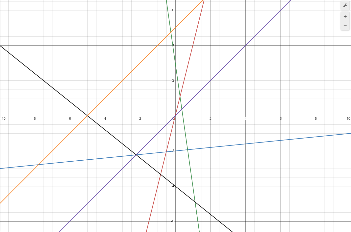
https://www.desmos.com/calculator/txjn03ol2e

When examining velocity curves, lines with steeper slopes indicate greater acceleration. A velocity curve with a slope of 2.5 would indicate a 2.5m/s/s acceleration, while a line with a slope of 10 indicates an acceleration of 10m/s/s. Readers who are familiar with calculus may have noticed the relationship between acceleration and velocity seems to be a derivative-integral one. Acceleration is the derivative of velocity, and velocity is the derivative of acceleration. Expressed mathematically these are

$a=\frac{d}{dt}(v_i+at)\\\\\\ v=\int a\ dt=(v_i+at)dt$

where

$v_i=initial\ velocity$

This post will not be making exclusive use of calculus, and will present it as needed for completeness.

Determining Displacement
One might think under an acceleration of 5m/s/s, the displacement of the object after one second is 5m. Is this indeed the case, and how would this question be answered? The easiest way to figure this out is to perform an experiment; however, we do not yet know how to accurately apply a constant acceleration to an object. Because the displacement and time of travel are known, a process of trial and error can be used, in which an angled track is set up to allow an object to slide down it. Suppose the track is 10m in length, and the inclination of the track can be adjusted to make it more or less steep. Figure 1 shows the basic setup.

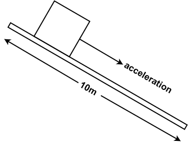
Figure 1 - Method to find position for acceleration of 5m/s/s

The object is released at the top of the track then one end of the track is elevated until the object starts to slide down it. When the object starts to move, a timer is started and the object's position relative to the top of the track is recorded at uniform time intervals. A 30 degree angle would be needed for a 5m/s/s acceleration, but more on that in another post. If this is done with a time interval of 0.5s over a period of 2s, the following data points are noted

Table 3 - Experiment data points

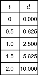
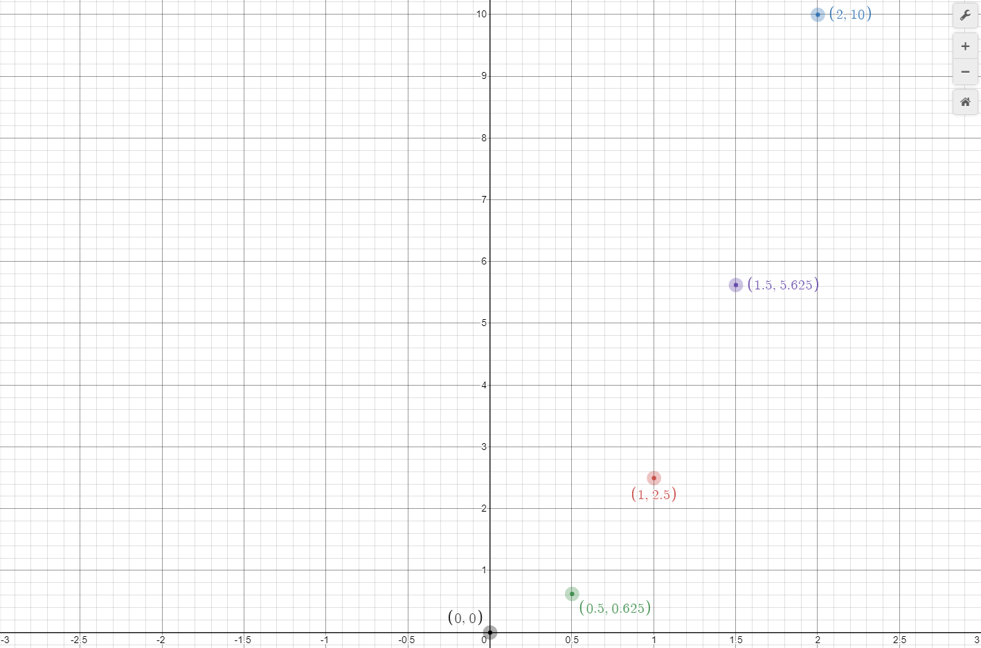
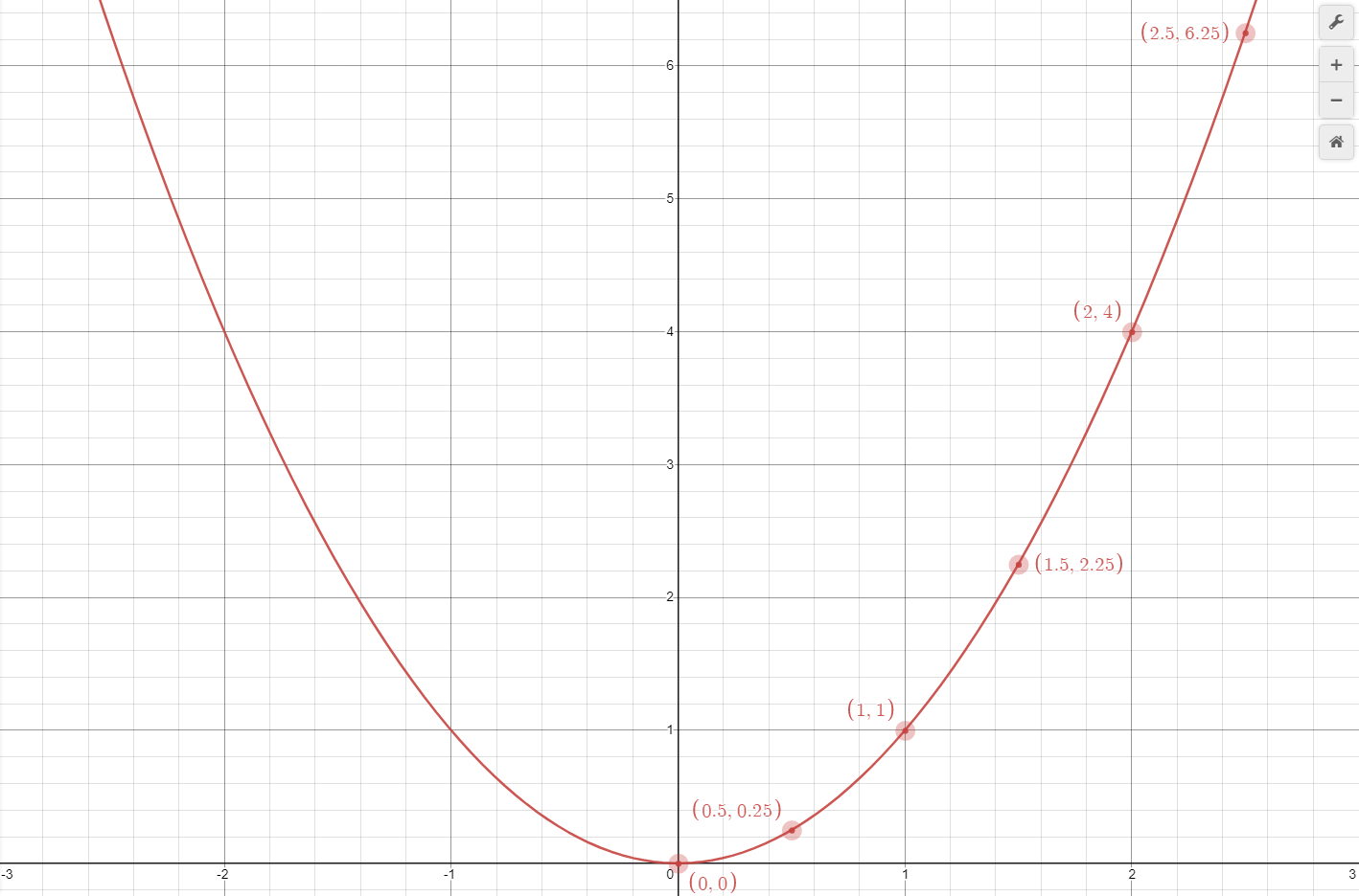
Graph 5 shows these data points plotted on a graph, and it is immediately evident the curve these points form is not linear, it is not a straight line. It is very often important in STEM to be able to recognize graphs of various types of curves and their respective functions. These data points appear to form half a parabola.

Graph 5 - Displacement data points for 5m/s/s acceleration

Parabolic curves are defined by functions containing a variable raised to an even power, and specifically for this example, a variable raised to the power of two. This type of function and curve are called quadratics. Another type of function, where the variable is raised to the third power, is known as a cubic. Curves for both these functions are shown in Graph 6.

Graph 6 - Quadratic and cubic curves
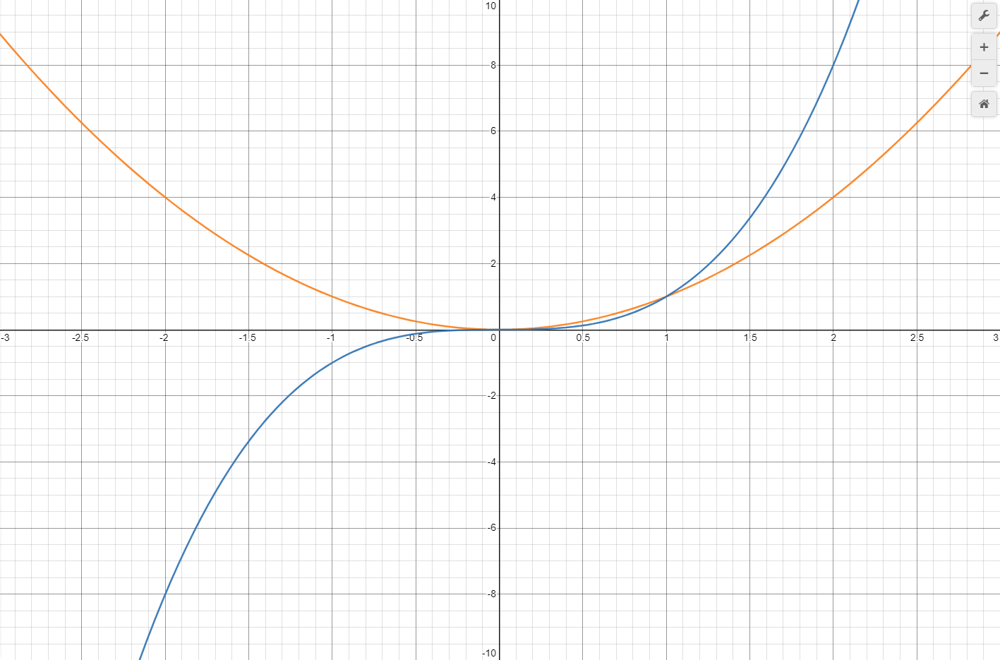
https://www.desmos.com/calculator/wcyepghybz

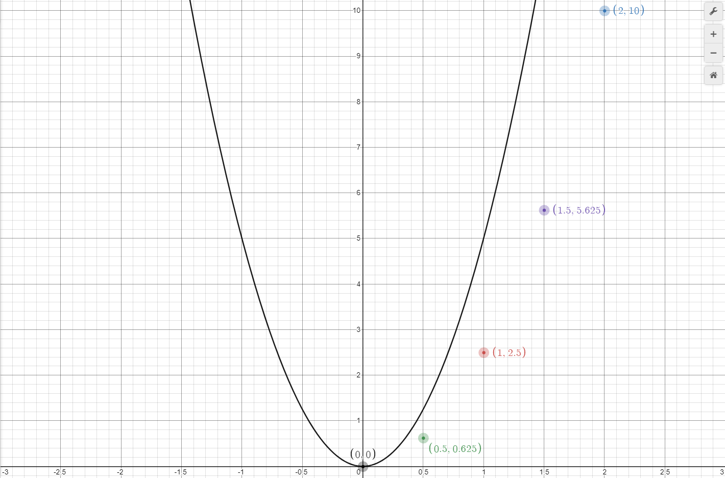
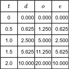
Plotting a basic quadratic function, shown below, against the displacement data results in Graph 7. This curve does not seem to fit, the only data point it goes through is (0, 0). By examining the error, calculated by subtracting the expected result from the observed result, we can determine the curve's y-values (displacement, s) are twice what they should be. This can be fixed by multiplying the curve's function by one half. Table 4 shows a table containing the error versus observed numbers.

$s=5t^2$

Graph 7 - Basic quadratic versus position data points

Table 4 - Error for basic quadratic versus data

Therefore, the function describing the displacement at time t of an object under an acceleration of 5m/s/s is given by

$s=\frac{1}{2}5t^2$

and the general form for displacement at time t with any constant acceleration is

$s=\frac{1}{2}at^2$

Graph 8 - Displacement curve

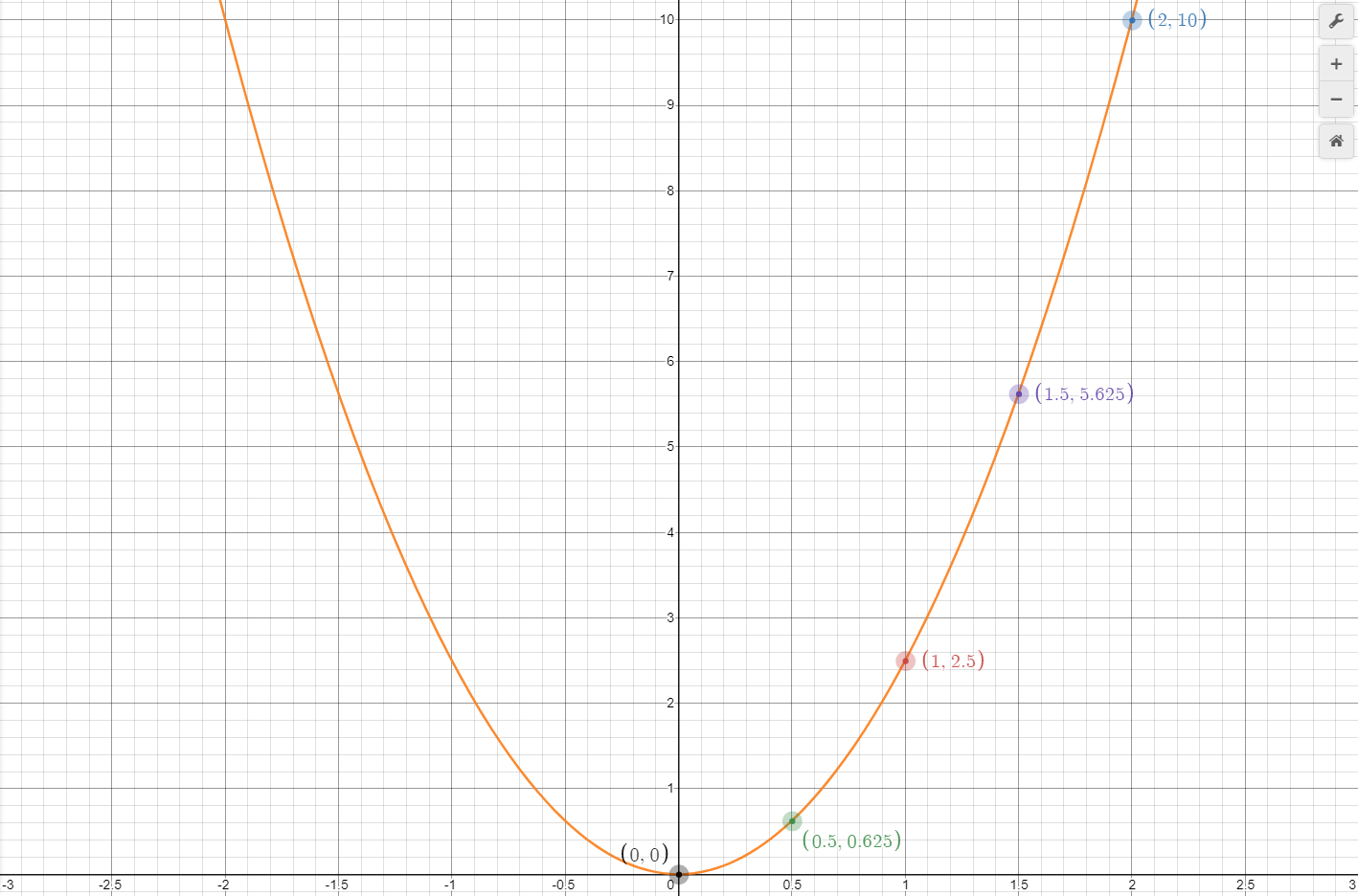
Graph 8 shows the new curve drawn with the data points, and it matches perfectly. We have just derived the formulas describing the behavior of an object under constant accelertion, and we did it without using calculus. Readers familiar with calculus may have again recognized a integral-derivative relationship here, this time between displacement and velocity. Displacement is the integral of velocity, and velocity is the derivative of displacement, as expressed below.

$s=\int v\ dt=\int (v_i+at)=s_i+v_it+\frac{1}{2}at^2\\\\\\v=\frac{d}{dt}(s_i+v_it+\frac{1}{2}at^2)=v_i+at$

Comparing Another Object
The object in the above example was accelerated at 5m/s/s and started with a velocity and distance of zero. Let's call this object "Object A". What would the graphs and equations look like if the object started with a velocity of 2.5m/s? Let's call this object "Object B". The initial velocity would need to be added to the acceleration term to get the velocity at any point in time. The function describing this is shown below.

$v=v_i+at=2.5+5t$

Graph 9 - Starting velocity of 2.5m/s versus 0m/s

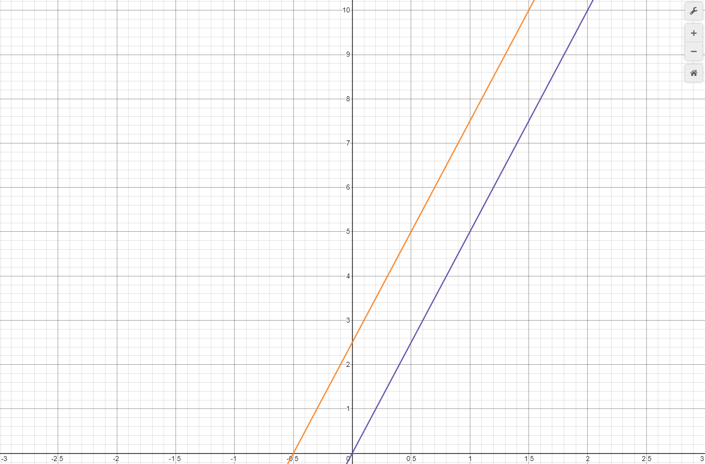
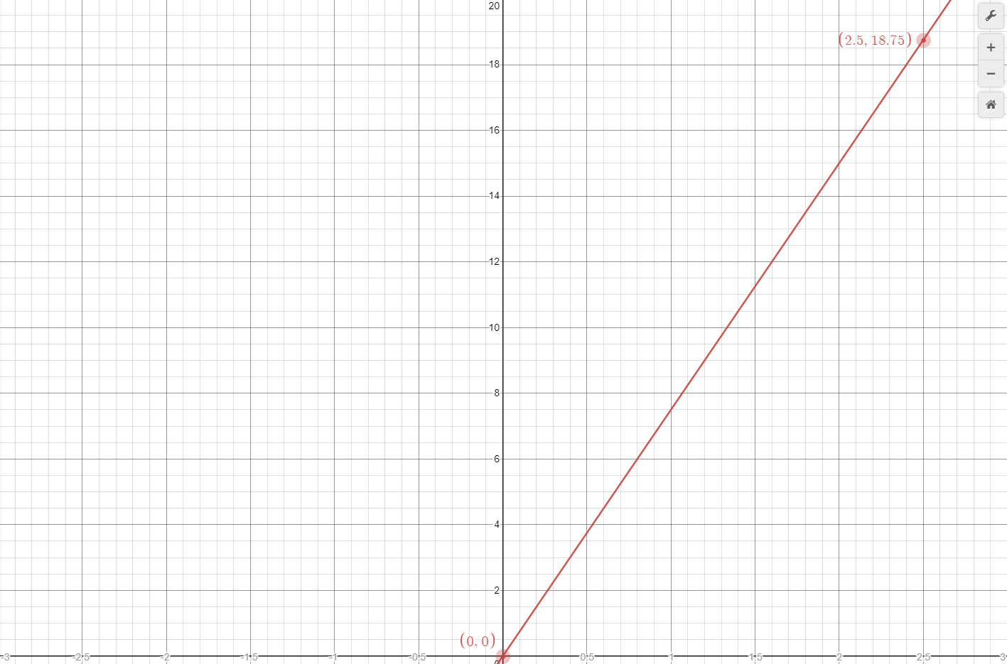
Graph 9 shows Object B's velocity plotted in orange against the velocity of Object A (in purple). The slopes are identical but Object B's velocity curve starts at y = 2.5 rather than y = 0. This matches the initial velocity of 2.5m/s as well as a 5m/s/s acceleration. We would also expect Object B's velocity at any point in time to be 2.5m/s greater than Object A's velocity at the same time.

What would the displacement graph look like in this situation? Because the Object B is starting with an initial velocity, its displacement curve should have greater distance values than Object A at each instant in time. Its displacement curve should also have the same shape as Object A's displacement curve. Graph 10 shows Object B's displacement versus Object A's displacement. The function describing this curve is shown below.

$s=s_i+v_it+\frac{1}{2}at^2=0+2.5t+\frac{1}{2}5t^2$

Graph 10 - Displacement for starting velocity of 2.5m versus 0m

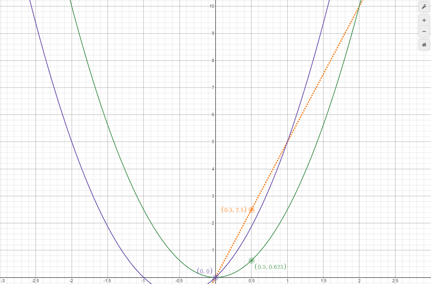
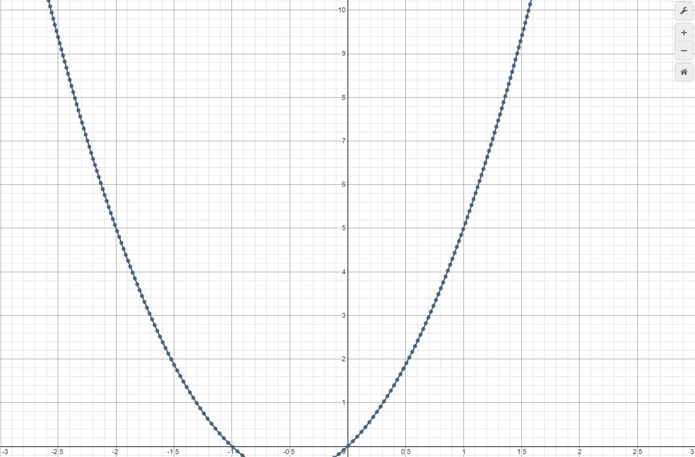
So far Object B's curve, in purple, matches what is expected with respect to Object A's curve, shown in green. Additionally, if Object A's displacement curve is moved along the graph's x and y axis by the proper amounts, the two displacement curves should match exactly. How can the correct amount of shift be determined? If the time at which Object A's velocity is 2.5m/s is noted by examining that object's velocity curve (the dotted orange line), the corresponding point on Object A's displacement curve can be marked. This has been done by marking the point on the object's velocity curve, in orange, then marking the corresponding point on the object's displacement curve. This point is at (0.5, 0.625), thus by shifting the curve in the opposite direction by these amounts, it should match Object B's displacement curve. Graph 11 shows the result of doing this shift. Object a's curve is represented by the dotted green line, and Object B's curve is represented in purple. They both match exactly.

Graph 11 - Displacement curves after shift

Now consider a situation where an object starts with zero velocity and a displacement of 2.5m. We would expect no change in the velocity curve, but would expect the displacement curve to be shifted up by 2.5. The function shown below describes this situation, and Graph 12 illustrates the resulting curve.

$s=s_i+v_it+\frac{1}{2}at^2=2.5+0t+\frac{1}{2}5t^2$

Graph 12 - Displacement curves for initial distance of 2.5m versus 0m

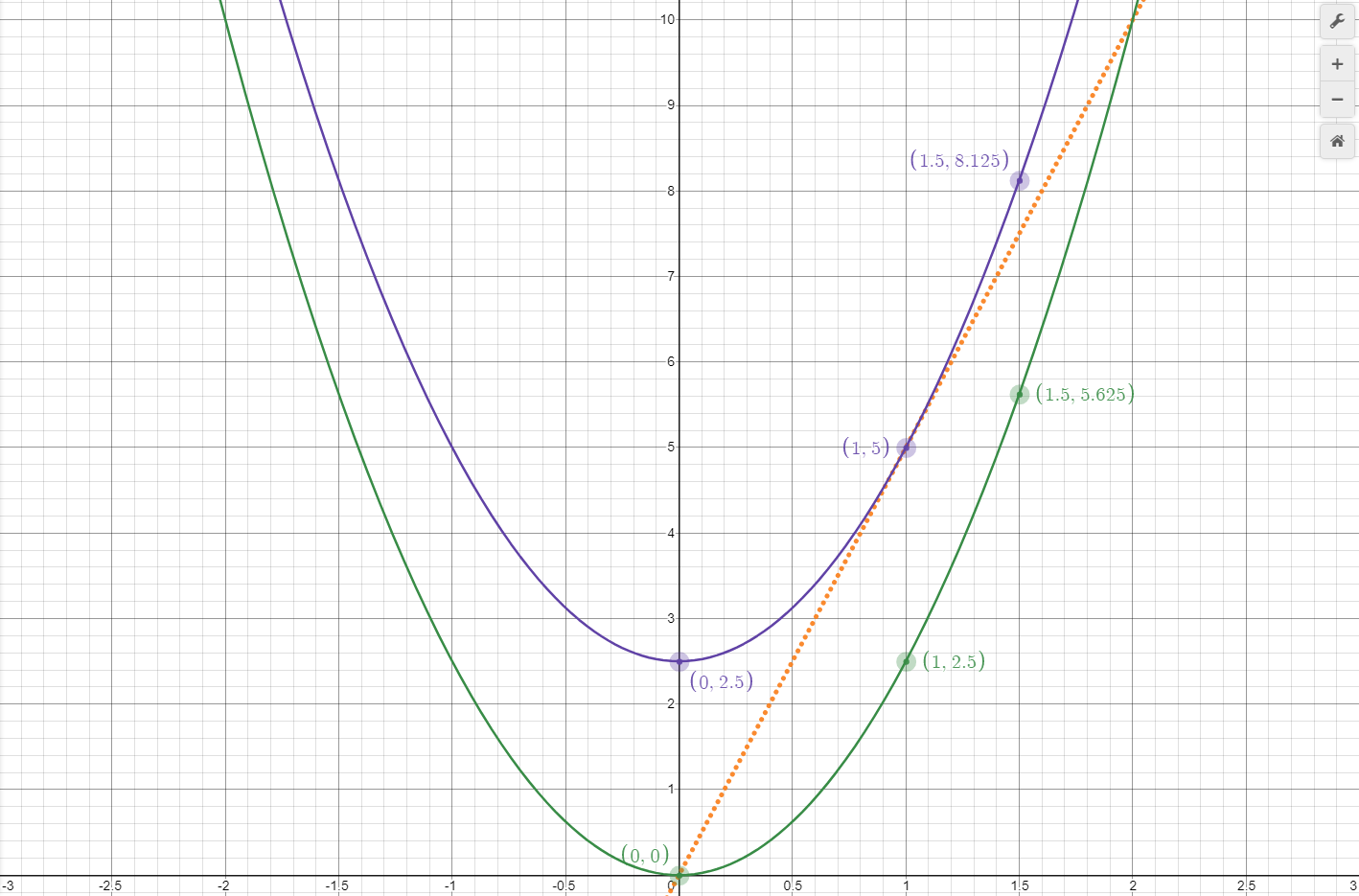
The curve shown in purple matches exactly the original curve shown in green, except it is shifted up by 2.5, indicating an initial displacement of 2.5m.

Useful Equations

Basic values

$\\s=s_f-s_i\\\\t=t_f-t_i\\\\v=v_f-v_i$

When displacement (s) is unknown

$\\a=\frac{v_f-v_i}{t}\\\\\\t=\frac{v_f-v_i}{a}\\\\\\v_i=v_f-at\\\\\\v_f=v_i+at$

When time (t) is unknown

$\\a=\frac{v_f^2-v_i^2}{2s}\\\\\\s=\frac{v_f^2-v_i^2}{2a}\\\\\\v_i=\sqrt{v_f^2-2as}\\\\\\v_f=\sqrt{v_i^2+2as}$

When final velocity (vf) is unknown

$\\a=\frac{2(s-v_it)}{t^2}\\\\\\s=\frac{1}{2}at^2+v_it\\\\\\s_f=\frac{1}{2}at^2+v_it+s_i\\\\\\s_i=\frac{1}{2}at^2+v_it-s_f\\\\\\t=\frac{-v_i+\sqrt{v_i^2-2as}}{a}\\\\\\v_i=\frac{2s-at^2}{2t}$

Sanity Checks
When using the above formulas it is important to check results to make sure they are sane. For example, suppose the answer to a problem of a driver applying a vehicle's brakes until it stops results in a negative acceleration, and after further calculations to find the distance the vehicle needed to stop, the distance is negative. A sane answer in this case would be to understand the result is a displacement from the vehicle's original position, and simply drop the negative sign to convert it to distance (the vehicle's initial position when the brakes were applied was 0 and subtracting the final [negative] displacement from zero results in a positive distance).

Getting a Bit Artsy

It is often useful to draw a diagram of what is happening when trying to understand how to go about solving a problem. List the information you have, the information you being asked for, and the information you will need to figure out to help solve the problem. Sometimes you will need to perform intermediate calculations to get information to solve the problem.

For example:
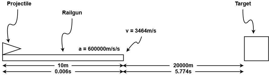
A 10m long railgun can accelerate an projectile at 600000m/s/s. How long would it take, to the nearest millisecond, a projectile shot by the railgun to reach a target 20km away, and how fast would it be going when it hit the target?

Begin by drawing a diagram and listing all the known information

Next convert any non-standard units to standard units. In this case 20km becomes 20000m

Looking at the formulas presented above shows the question of projectile speed can be solved directly but time cannot, thus

$v_f=\sqrt{v_i^2+2as}=\sqrt{0^2+2\times 600000\times 10}=\sqrt{12000000}=3464m/s$

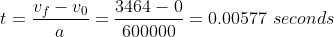
By the time the projectile leaves the railgun it will have been accelerated to 3464m/s. This information can be used to calculate the time of flight

$t=\frac{s}{v}=\frac{20000}{3464}=5.774\ seconds$

The problem is not finished yet because this is only the time it takes the projectile to reach to target after is has left the railgun. The time it took to be accelerated by the railgun must be calculated and added to the above result.

$t=\frac{v_f-v_0}{a}=\frac{3464-0}{600000}=0.00577\ seconds$

Therefore, the total time is 5.774s + 0.006s, or 5.78s.

Try It Yourself

Here are some problems for you to try solving. Answers will be at the end of the next week's physics post.

a. What is the velocity of a satellite that travels 75km in 10s?
b. How far will the satellite travel in 60s?
c. What would the satellite's acceleration be if its velocity increased by 500m/s over a period of 50s?
d. What would its final velocity be after this acceleration?
e. What functions describe the car's acceleration, velocity, and distance? What do the curves of each look like when graphed?
a. A bullet is shot from a rifle having a 0.5m long barrel. If the bullet's velocity is 600m/s when it leaves the barrel, what is its acceleration?
b. How long did it take the bullet to leave the barrel?
c. Calculate the values for a and b if the barrel's length was 0.75m.
d. What functions describe the bullet's acceleration, velocity, and distance? What do the curves of each look like when graphed?
a. A train sits stopped 15km from a city at 10:00am. If the train has a top speed of 100km/h and can accelerate at 0.1m/s/s, what time would the train reach the city at maximum speed?
b. How much time would it take the train to accelerate to maximum speed?
c. How far would the train travel while moving at its maximum speed?
d. What functions describe the train's acceleration, velocity, and distance? What do the curves of each look like when graphed?
a. The velocity of an aircraft is 250m/s at 9:30am and 260m/s at 9:31am. How far did it travel during that time?
b. What was its acceleration during that time?
c. What functions describe the aircraft's acceleration, velocity, and distance? What do the curves of each look like when graphed?
a. A car is moving at 25m/s when the car's driver applies the brakes. What is the car's acceleration if the car comes to a stop in 2.5s?
b. How far does the car travel during these 2.5 seconds?
c. What functions describe the car's acceleration, velocity, and distance? What do the curves of each look like when graphed?
a. A projectile is shot from a vertically mounted gun that is 2m long. It leaves the gun with a velocity of 500m/s. How high does the projectile go?
b. How long does it take the projectile to hit to the ground after the gun's trigger is pulled?
c. What was the acceleration of the projectile while in the gun?
d. What is the projectile's velocity when it hits the ground?
e. What functions describe the car's acceleration, velocity, and distance? What do the curves of each look like when graphed?
a. Determine the acceleration and velocity using the graph below
b. Draw the acceleration and velocity curves from 0.0 to 2.5 seconds
c. Determine the functions for the acceleration and velocity
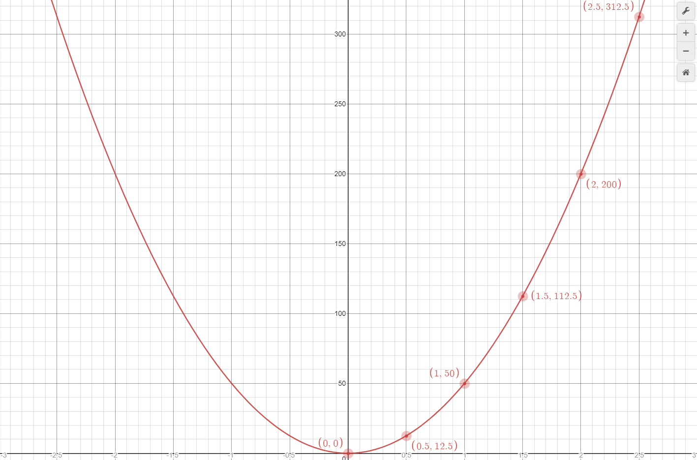
a. Determine the acceleration, and position at 0, 0.5, 1.0, 1.5, 2.0, and 2.5 seconds using the graph below
b. Draw the acceleration and position curves from 0.0 to 2.5 seconds
c. Determine the functions for the acceleration and position
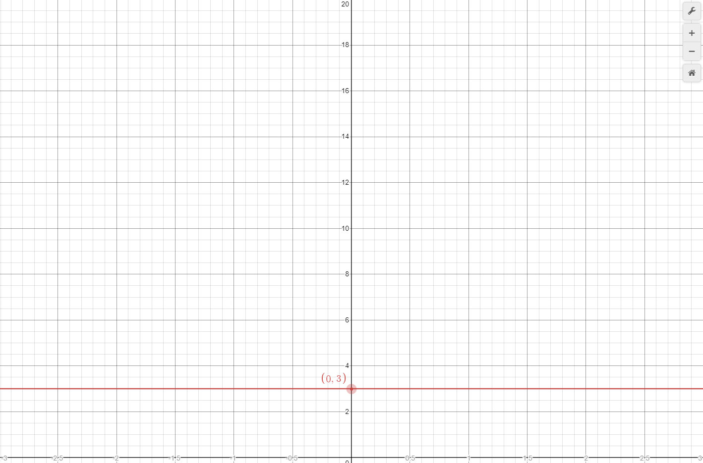
a. Determine the acceleration and velocity using the graph below
b. Draw the acceleration and velocity curves from 0.0 to 2.5 seconds
c. Determine the functions for the acceleration and velocity
a. Determine the position, and velocity at 0, 0.5, 1.0, 1.5, 2.0, and 2.5 seconds using the graph below
b. Draw the velocity and position curves from 0.0 to 2.5 seconds
c. Determine the functions for the velocity and position

Posted with STEMGeeks

physics education stem

0.000

0 comments