Mathematics - All About Solving Polynomials (part 3)

over 2 years ago

Introduction

Hey it's a me again @drifter1!

Today's article is another high-school refresher on Mathematics, and more specifically on Solving Polynomials. This is the third and final part. I highly suggest checking out part 1 and part 2 before this part!

So, without further ado, let's get straight into it!

Divide by Factor

After applying the Rational Root Test, and either by brute force substitution of the candidates or using some division algorithm, it may be possible to find out that some rational number r is a root. Based on the Factor Theorem this means that x - r is a factor of the polynomial.

If only brute-force was used then the polynomial will have to be divided by that factor in order to end up with a reduced polynomial that will give the remaining roots / factors. Of course, dividing by each candidate factor is more efficient, because the reduced polynomial is produced as a side-product directly!

Two main techniques can be used for dividing. The first one, known as polynomial long division, applies for any polynomial division with a divisor that has the same or lower degree than the dividend. The second one, known as synthetic division, can also be generalized for any division, but is more commonly used for divisions by linear monic polynomials of the form x - a.

Polynomial Long Division

Polynomial long division is a type of Euclidean division of polynomials. Starting off with two polynomials, A and B, and if B is not zero and is of same or lower degree than A, there will be a quotient Q and a remainder R, so that:

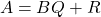
Of course R must be either 0 or of lower degree than B.

R = 0 basically means that B is a factor of A, and is exactly what is checked for when trying out the possible rational root candidates!

Short Division

When applied on pen-and-paper, the Blomqvist's method, also known as short division, can be used instead, which requires less writing and is faster as remainders are determined mentally.

The steps are as follows:

Write The dividend at the top and the divisor below it, and put a bar below them, where the quotient will be written from left to right later on.
Divide the first (highest degree) term of the dividend by the first (highest degree) term of the divisor. Place the result below the bar. Multiply that result with the second term of the divisor and determine the partial remainder by subtracting that value from the second term. Mark that first term of the dividend as used and replace the second term with the corresponding new remainder calculated. That way the dividend basically gets replaced by the remainder.
Repeatedly, divide the highest term of the remainder by the highest term of the divisor. Apply the previous steps again until the remainder has a smaller degree than the divisor.
The result of division can be thought of as the quotient (below the bar) times the divisor plus the remainder.

Simple Example

Let's get into a simple example to understand the procedure better!

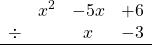
Dividing the first term of the dividend, x², by the first term of the divisor, x, gives x, which is put below the bar. Multiplying this result by the second term of the divisor, -3, gives us -3x, which when subtracted from the second term of the dividend, -5x, results in -5x -(-3x) = -2x. So, now the first term can be striked out, and the second term replaced by the calculated remainder -2x.

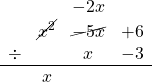
Dividing the first term of the remainder, -2x, by the first term of the divisor, x, gives -2, which is put below the bar. Multiplying it by the second term of the divisor, -3, gives (-2)(-3) = 6, which when subtracted from the second term of the remainder, 6, gives 6 - 6 = 0. So, the new remainder is 0 and the division has been completed.

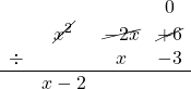
In other words, applying polynomial division it was proven that 3 is a root of the polynomial equation, or that x - 3 is a factor of the polynomial. Additionally, the quotient x - 2 gives us the second root, which is x = 2.

The polynomial can be factorized as follows:

Synthetic Division

Regular synthetic division, which is also known as Ruffini's rule, applies to division by polynomials of the form x - a. The main advantages of this approach are:

no variables are written
few calculations are performed
sign errors are prevented by converting subtractions to additions
little paper space is required (when compared to long division)

So, this technique is basically made for solving polynomials!

Let's first try to understand the concept and why it works.

Nested Multiplication

Synthetic division is based on something known as nested multiplication. When substituting each root candidate quite a lot of multiplications and additions are required if the calculations are applied on the polynomial as they come up. But, if the polynomial gets written in nested multiplication format then the number of multiplications and additions becomes far less. This allows for faster calculations and the benefit adds up really fast for higher-degree polynomials.

For example, consider the following polynomial:

From the Rational Root Test, the root candidates are ±1, ±2, ±4, up to ±32.

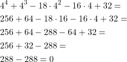
Trying out x = 1 is simple, as there are no difficult multiplications (one term is 1ⁿ = 1), and in that case nested multiplication is not required:

So, let's say that we instead had to try out x = 4, because the previous candidates where not roots. In that case the multiplications and additions pile up by quite a margin, even if the exponentials of 4 are calculated before-hand:

Thus, let's write the polynomial in nested multiplication format:

and calculate x = 4 on that:

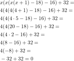
Only 4 additions and 3 multiplications are required for that calculation, and those calculations where also much simpler (no exponentials which yielded additions with bigger numbers) and faster!

Writing Format

Of course, we promised that no variables will be required! So, how does one write the nested multiplication in a better format?

Synthetic division is written as follows:

Write only the coefficients of the polynomial, including the zero coefficients. Draw a line on either side and put the root candidate there (not the factor!). Finish up with a line below.
Bring down the first coefficient directly.
Repeatedly multiply the result (first coefficient in the first iteration) by the candidate and add to the top line.
If the right-most result is zero then the candidate is a root.

Let's take a look at the previous example again by using that approach in order to check if 4 is a root.

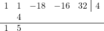
The calculation goes as follows:

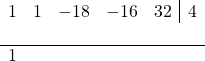
Now the initial result 1 is multiplied by the candidate root 4 and added to the second coefficient, 1, giving 5.

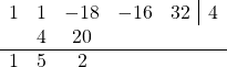
Multiplying 5 by 4 gives 20 which is added to the third coefficient, -18, resulting in 2.

Repeating the same method for the remaining two coefficients, the final result is:

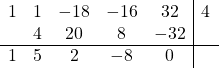
The right-most result is 0, which means that x = 4 is a root!

The result is equal to the coefficients of the reduced polynomial, which in that case is:

Applying the same technique on that polynomial once again, will reduce the degree once more, yieling a quadratic polynomial that can be solved directly!

Root Boundary Techniques

There are some additional theorems that can be used together with the Rational Root Theorem and Synthetic Division to help narrow down the search even further, these are:

Intermediate Value Theorem:
- If the graph of the polynomial is above the x-axis for one value of x (positive) and below the x-axis for another value of x (negative), then it must cross the x-axis somewhere between (zero).
- Using it its possible to identify where roots will surely exist, but not where there are no roots!
Upper and Lower Bounds:
- Applying the Synthetic Division technique for a root or non-root number may also give additional information for where the roots actually reside.
- If the result of Synthetic Division by a positive number, yields only positive values or zeroes in the bottom row, then that number is an upper bound of the roots.
- If the result of Synthetic Division by a negative number, yields alternating signs in the bottom row, then that number is a lower bound of the roots.

Irrational Roots - Numerical Methods

When no more rational roots can be found, then the irrational roots can be found approximately by applying numerical methods. In general these methods can be thought of as root-finding algorithms. It's part of a whole branch of mathematics known as Numerical Analysis.

There are various types of methods, such as:

Bracketing methods which rely on the Intermediate Value Theorem
Iterative methods, such as Newton's derivative-based method, Secant's method, Steffensen's method or Inverse Interpolation.

These topics are of course far more advanced, and no longer high school math, which was the main target of this series! For example, I had a Numerical analysis course during my CS studies. A series on such topics is on my to-do list for sure...

RESOURCES:

References

Mathematical equations used in this article, have been generated using quicklatex.

Block diagrams and other visualizations were made using draw.io.

Final words | Next up

And this is actually it for today's post!

The next article(s) will be about:

Exponentials, Roots and Logarithms

Basically more High-School Math Refreshers!

See ya!

Keep on drifting!

Posted with STEMGeeks

mathematics science education algebra polynomials solving roots factors division stem

0.000

0 comments