Goal Seek Function In Excel
Hi there. In this post, I cover the goal seek function in Excel with examples. Goal seek is a useful tool in Microsoft Excel for doing algebra and solving unknowns in Excel.
Screenshots are Excel snapshots and math text is rendered in Latex with Quicklatex.com.

The Goal Seek Function In Excel
Mathematics calculations done with pencil and paper is much more different than doing mathematics with the use of software. Microsoft Excel is a spreadsheet software where users can input data in the form of numbers, text and/or symbols. It is great with built-in formulae for doing mathematics calculations for inputting values on blank cells or changing values.
The Goal Seek function in Excel is great for solving for unknown values given that there is a formula provided in a cell. Goal Seek can be found in the Data tab and in What-If Analysis. Note that I am using Microsoft 2013.
Examples
I showcase three examples where Goal Seek can be used.
Example One: Profit = Revenue - Expenses
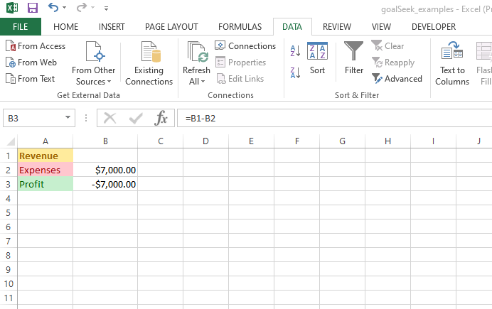
In this simple example, Goal seek is used to determine the expense amount given a fixed revenue amount. The formula for profit is Revenue minus Expenses. In Excel the profit formula is =B1-B2.
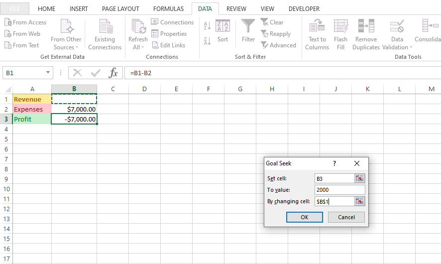
In this example I want to determine the revenue amount that is associated with an expense amount of $7000 in order to obtain a profit of $2000. To access the Goal Seek function tool, go to Data then click on What-If Analysis. The set cell is B3 which is the cell associated with profit. Set the value in To value: to 2000 as in 2000 profit. In the By changing cell: select the cell in which Goal Seek will output which is the Revenue cell of B1.
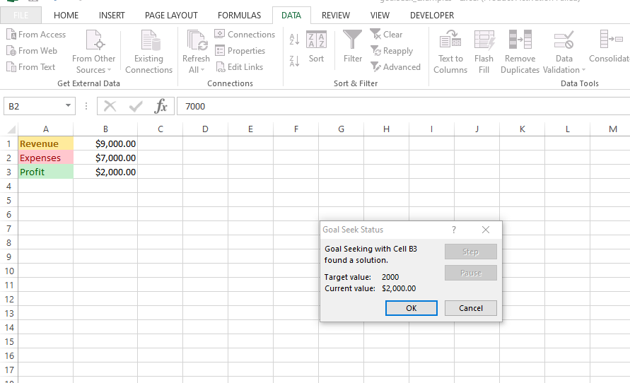
Once the OK button is clicked, the Goal Seek function does the necessary calculations to solve for the unknown revenue value. The unknown revenue value turns into 9000 which is associated with a 7000 expense amount and a 2000 profit amount. There!
Example Two: Test Scores
The Goal Seek examples online through search engine results usually have an example of test scores where you find out what grade you need on a test or course to get a certain overall average. This example is nice but it does assume that everything is weighted equally. If there are 5 tests in a course then every test is worth 20% each. This equal weighting of tests & assignments is not realistic.
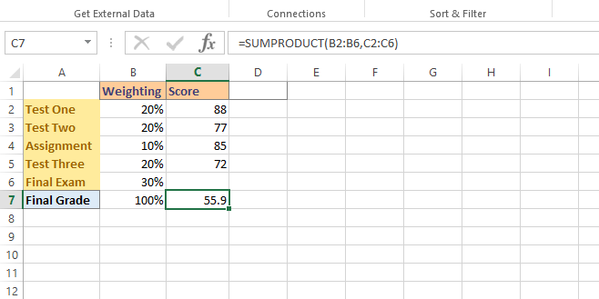
In this second example I feature a student's scores for a course where there are tests, one assignment and a final exam. The tests and assignments are weighted at 20% each, the assignment is worth 10% and a final exam has a 30% weighting. The first screenshot features the student's scores so far in the course before the final exam.
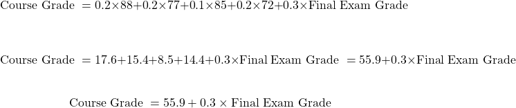
If everything is weighted equally the formula for the final grade would involve the usual average. That is adding up all the scores and dividing by the number of tests & assignments.
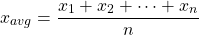
In this example, a test is not weighted the same as an assignment or a final exam. A dot product is needed here. In Excel, the dot product can be done with =SUMPRODUCT(B2:B6,C2:C6).
This sum product does this calculation.
Suppose this student was a course grade of 77. What final exam grade does the student need to obtain a course grade of 77? This final exam grade score can be found with calculations by hand or with the use of Excel's goal seek tool.
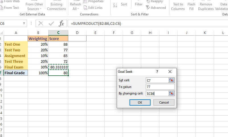
In the Goal Seek tool, set the cell to C7 which is the cell for the final grade for the course. For To value set the number to 77. In By changing cell select the cell for the unknown variable/value which is cell C6. Cell C6 associated with the final exam score.
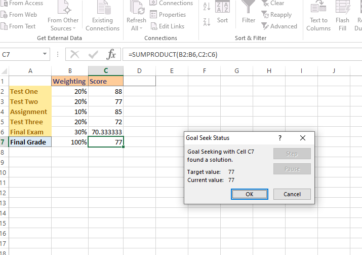
Once you click OK, the Goal seek tool does its calculations and fill in the value for the final exam score. To obtain a final course grade of 77, the student needs to score of 70.33% on the final exam. This seems highly attainable for the student assuming no crazy surprises on the final exam.
Example Three: Compound Interest
This example features a single investment with the power of compound interest. Given an initial investment (P), the number of periods (n) and an interest rate (i) we have this formula for the amount of this investment in the future (F) after n periods
In this example the interest rate is the annual interest rate divided by 12. This division by 12 is the interest rate for the one month period as each period is one month. Two years is the same as 24 monthly periods.
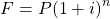
In Excel, I have the compound interest formula as =B1*(1 + $B$3/12)^B2. Cell B1 is the initial investment. B2 is the number of compounding periods. Cell B3 is the annual interest rate before being divided by 12.
What annual interest rate is needed for an initial investment of $2000 over 2 years (24 months)? Do assume compound interest.
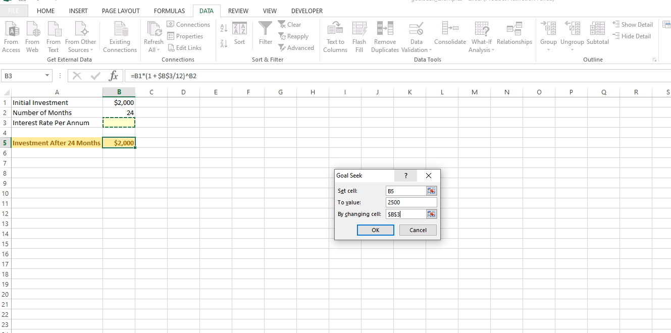
Under Excel's Goal Seek tool, set the cell to B5. The value for B5 is 2500 for the future value of the investment. For the By changing cell part set the cell to B3 which is associated to the interest rate we are solving for.
Clicking OK here will yield an annual interest rate of 11.21%. This 11.21% or 0.1121 is for the variable i.

Posted with STEMGeeks