Combining IF & Stats Functions In Excel

Hi there. In this post, I showcase combining if statements along with statistics functions in Microsoft Excel.

Topics

Excel's Statistical Functions
Sample Excel Dataset
Combining IF & Stats Functions

Excel's Statistical Functions

Excel does contain a good handful of summary statistics functions. The function =AVERAGE() is for computing sample means, =MEDIAN() is for sample medians, =MODE() is for finding the most frequent value in a list of numbers, =VAR.S() is for sample variances and STDEV.S() is for sample standard deviations.

You also have skewness and kurtosis represented by =SKEW() and =KURT() respectively.

From the Excel functions mentioned above only the =AVERAGE() has a version that uses an if conditional statement. The function =AVERAGEIF() if for computing an average that meets a certain condition. For multiple conditions, use =AVERAGEIFS(). There are no if versions for the mode, median, variance and standard deviations in Microsoft Excel 2013. A workaround solution is to combine Excel's =IF() function along with the desired statistical function.

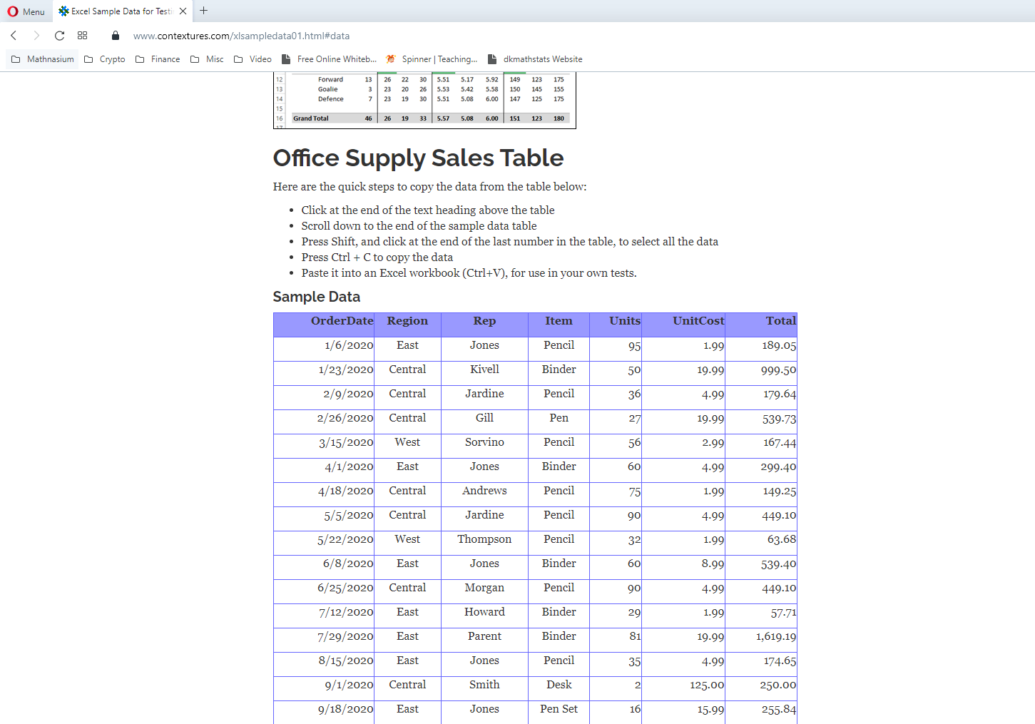
Sample Excel Dataset

The sample dataset is from the Contextures.com website. This data is based on office supply sales. The table can be copied and pasted into Excel.

Combining IF & Stats Functions

I showcase a few examples of combining the if statement in Excel along with a statistical function. This also works for MAX(), MIN() and COUNT() functions. I use Excel 2013.

References:

Variance Of Total Sales By Item

Excel is nice when it comes to computing something like the variance of a list of numbers. Computing the variance by hand is time consuming and annoying so it is better to use software like Excel or programming tools like R, Python.

For the variances of total sales by item, I have a mini table. There are five rows for the item types for pencil, pen, binder, desk and pen set along with their variance values. I compute the variance for the total values corresponding to pencil, then the variance for pens and so on. There would be 5 variances in total here. (Screenshot below)

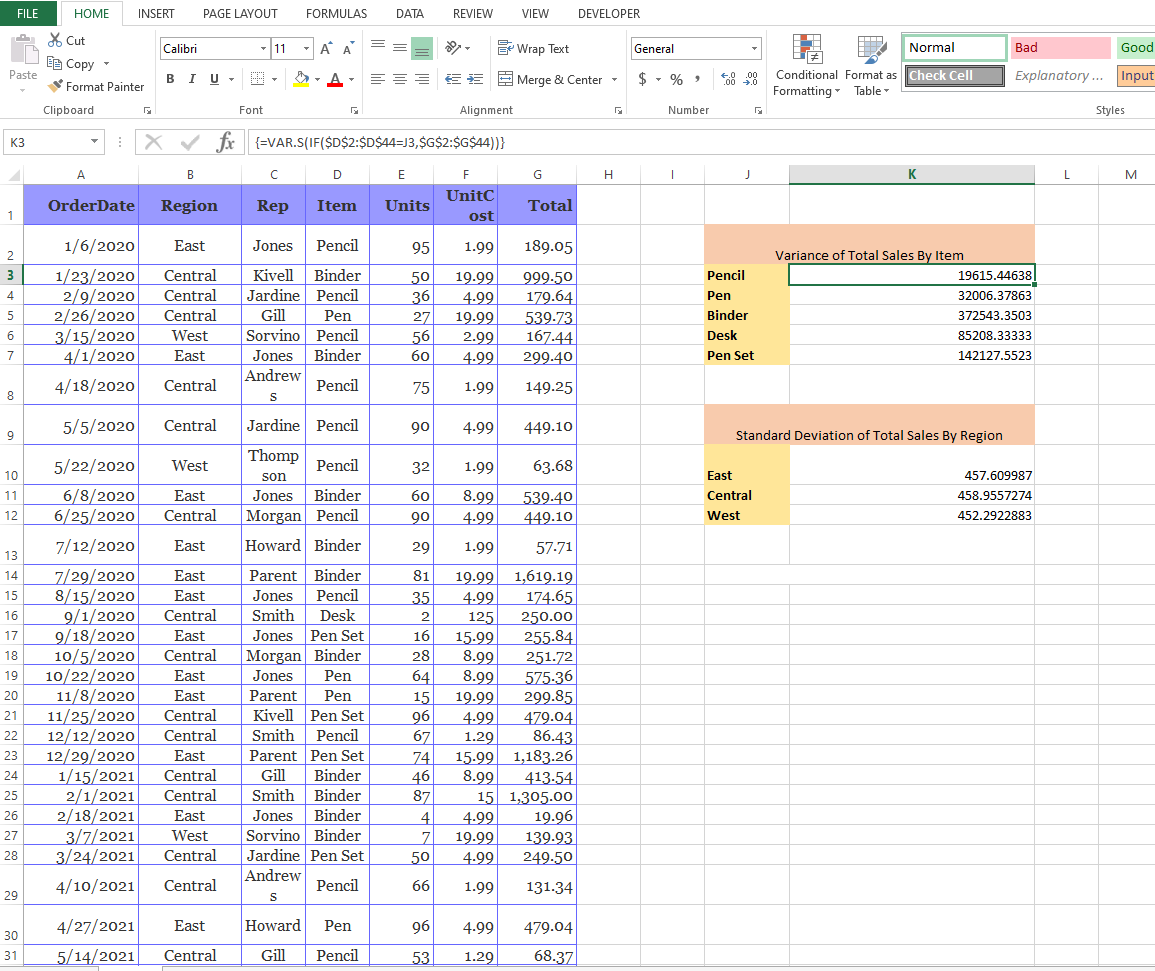
The item column in my Excel spreadsheet is D2:D44. This is column D with rows 2 to 44. The total sales column is G2:G44. Pencil text is in cell J3.

For the variance of total sales for pencils, the Excel command is =VAR.S(IF($D$2:$D$44=J3,$G$2:$G$44)). Do use CTRL+SHIFT+ENTER to wrap the formulae with curly brackets to ensure the variance values are shown.

The embedded IF statement is for filtering out the total sales that do not correspond to pencils. The logical test in the IF statement is $D$2:$D$44=J3. The total values that remain are the total sales for pencils that are used for the outside VAR.S Excel function for computing the sample variance.

I repeat the =VAR.S(IF($D$2:$D$44=J3,$G$2:$G$44)) function for the other item types. For the variance of pens do change it from J3 to J4 to obtain =VAR.S(IF($D$2:$D$44=J4,$G$2:$G$44)). Binder is with J5, desk is for J6 and pen set is with J7.

Note that the dollar signs is to hold the Item column & the total column in place when using the formula in other cells.

Standard Deviation Of Total Sales By Region

Computing the standard deviation with an embedded if statement is not much different than the one with sample variances. In this example, I do sample standard deviation of total sales by region.

The total column is still the same column as in G2:G44 for column G rows 2 to 44. We change from the Item column to the Region column. The region column is B2:B44. (Screenshot below)

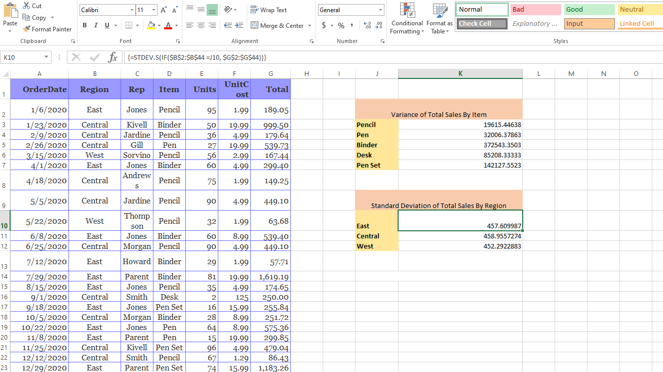
The formula for the standard deviation for the East region is =STDEV.S(IF($B$2:$B$44 =J10, $G$2:$G$44)). J10 refers the cell with the text East, J11 is for Central, J12 is for West.

Don't forget CTRL+SHIFT+ENTER when entering the formulae to show the values.

Thank you for reading.

Posted with STEMGeeks

References:

- https://www.educba.com/max-if-in-excel/
- https://www.ablebits.com/office-addins-blog/2019/10/30/excel-max-if-formula/