Ultimate Guide - Compare two lists or datasets in Excel
Hay Paula, can you compare lists in Excel?or
What is the best way to compare two sets of data in Excel?Very often there is a requirement in Excel to compare two lists, or two data sets to find missing or matching items. As this is Excel, there are always more than one way to do things, including comparing data. From formulas and Conditional Formatting to Power Query. In this article we are going to look at a number ways to compare two lists in Excel and we will also look at comparing entire rows of a data set.
Maybe your preferred way is not included below. If not why don’t you drop a comment below and share with us how you like to compare two lists or datasets in Excel. I look forward to reading your comments.
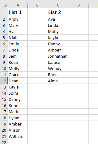
We wish to compare List 1 with List 2.
Contents
Quick Conditional Formatting to compare two columns of data
Clearing the Conditional Formatting
Match data in Excel using the MATCH function
Compare 2 lists in Excel 365 with MATCH or XMATCH as a Dynamic Array function
MATCH and Dynamic arrays to compare 2 lists
XMATCH Excel 365 to compare two lists
Tables – Comparing lists in Excel where the ranges sizes might change
Highlight differences in Lists using Custom Conditional Formatting
Copy formula to Custom Conditional Formatting
Other Formulas used to compare two lists in Excel
VLOOKUP to compare two lists in Excel
XLOOKUP to compare two lists in Excel
COUNTIF to compare two lists in Excel
How to compare 2 data sets in Excel
Comparing lists or datasets using Power Query

Take a FREE course with us
Quick Conditional Formatting to compare two columns of data
Conditional formatting will allow you to highlight a cells or range based on predefined criteria. The quickest and simplest way to visually compare these two columns quickly is to use the predefined highlight duplicate value rule.
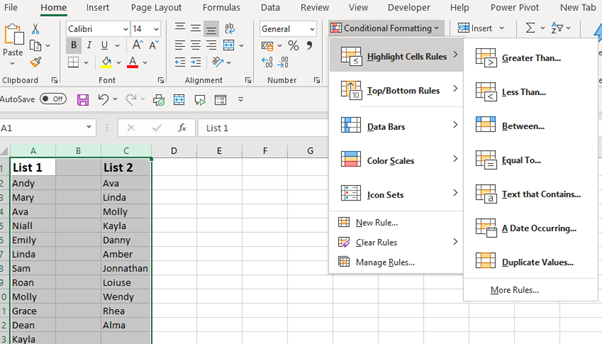
Start by selecting the two columns of data.
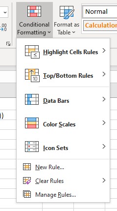
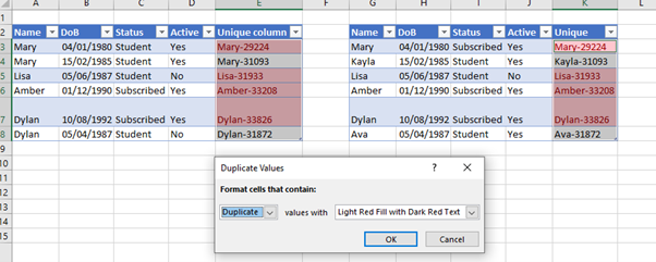
From the Home tab, select the Conditional Formatting drop down. Then select Highlight Cells Rules. Next select Duplicate values.
A Duplicate Values settings box will open where you can define the formatting and select between Duplicate or Unique values.
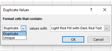
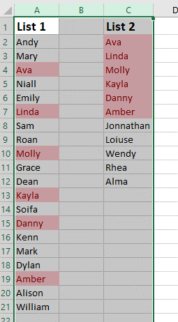
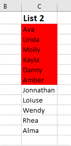
By Selecting Duplicate, all reoccurring entries will be set to the selected formatting. Now you can quickly see the items in List 1 that are in List 2 as these are the formatted items. You can also quickly see the items in list 2 that are not in list 1 as these do not have formatting applied.
However, you can also format the Unique items. This can be achieved by selecting Unique from the Duplicate Values setup box.
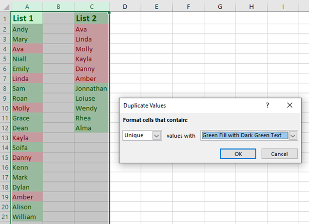
In this case, we have applied two different conditional formats. The red indicating the duplicates and the green indicating the unique items.
Note, I did not just take the cells with data, I grabbed all of columns A to C. Column B has no data, so it cannot affect the results. However, these cells do contain the conditional formatting applied so it would be better practice to only select the cells you need.
Clearing the Conditional Formatting
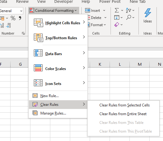
To clear all conditional formatting, first select the cell, or range. Then select the conditional formatting drop down on the Home ribbon. Next select Clear Rules. Finally Select Clear Rules from Selected Cells.
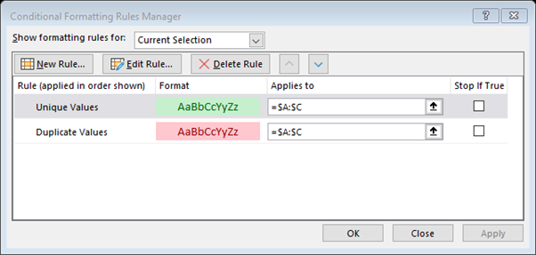
If you have more than one conditional formatting applied at once and you only want to remove one of these, select Manage Rules from the conditional formatting drop down. Select the rule you want to delete and then select Delete Rule.
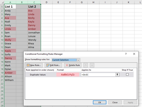
By pressing OK, the rule will removed from the Rules Manager and the cells will no longer contain the formatting.
So that is the most basic way you can compare two lists in Excel. Its quick, its simple and it is effective. You can also apply conditional formatting based on formulas, which we will look at later in this article.
Match data in Excel using the MATCH function
There are many lookup formulas that you can use to compare two ranges or lists in Excel. The first we will look at is the MATCH function.
The MATCH function returns the relative position in a list. A number based on its position, if found, in the lookup array.
The syntax for MATCH is
=MATCH (lookup value, Lookup array, Match type)
Where lookup value is the value you want to find a match for. Lookup array is the list in which you are looking for a match. And Match type allows you to select between an exact or approximate match.
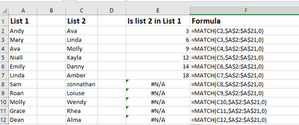
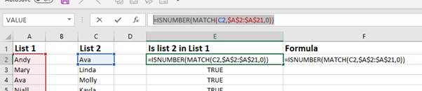
We want to write a match formula to see if the items in List 2 are in List 1.
In cell E3 we can enter the formula
=MATCH(C2, $A$2:$A$21,0)

By filling this formula down, for the values where Excel finds a match, the position of that match will be returned. Where there is no match the return value will be an #N/A.
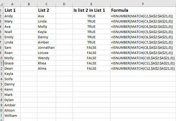
Very often, the relative position or the #N/A is of no value to us and we need to convert these values into true or false. To do this we can easily expand on our Match formula using a logical function. As Match returns a number, we can use the ISNUMBER function
=ISNUMBER(MATCH(C2, $A$2:$A$21,0))
Compare 2 lists in Excel 365 with MATCH or XMATCH as a Dynamic Array function
If you are using Excel 365 you have further alternatives when using MATCH to compare lists or data. As Excel 365 thinks in arrays, we can now pass an array as the lookup value of MATCH and our results will spill for us. This removes the need to copy the formula down and with only 1 formula, your spreadsheet will be less prone to errors and more compact.
MATCH and Dynamic arrays to compare 2 lists
If you are not yet familiar with Dynamic Arrays, I would suggest you have a read of this article: Excel Dynamic Arrays – A new way to model your Excel Spreadsheets: to get a better understand on how they work and spill ranges.
The only change to the match formula is instead of selecting cell C2 as our lookup value we will select the range C2:12
=ISNUMBER(MATCH (C2:C12,$A$2:$A$21,0))
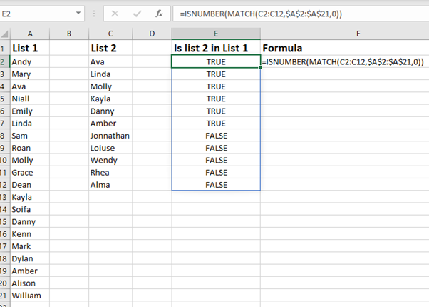
As you can see, the one formula spills the results down column E.
XMATCH Excel 365 to compare two lists
Excel 365 also introduces the new function XMATCH. Just like the MATCH function XMATCH returns a relative position in a list. Now you are familiar XLOOKUP, which replaces the old VLOOKUP function, you know XLOOKUP comes with additional power. This come in the form of new conditions in the formula syntax such as search mode and match types. Well, XMATCH also as this extra power over its predecessor MATCH.
The syntax for XMATCH is
XMATCH (Lookup Value, Lookup Array, [Match Mode],[Search Mode])
Where
Lookup Value is the value you are looking to find the relative position
Lookup Array is the row or column that contains the Lookup Value
Match mode is optional. Unlike the old MATCH function, the default is an exact match. You can also select between
- Exact match or next smallest
- Exact match or next largest
- Wildcard match
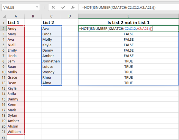
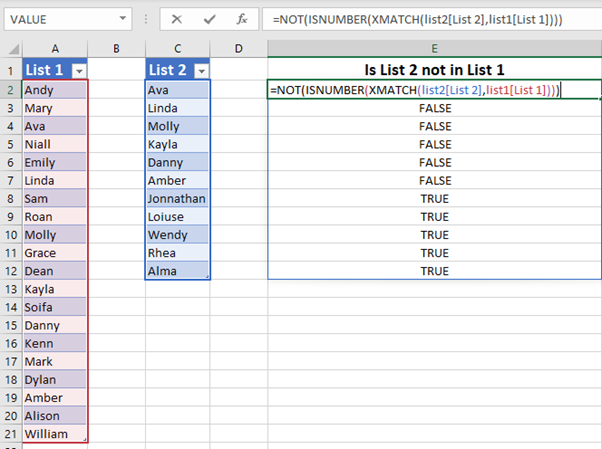
With XMATCH we can use either Dynamic arrays or cell references to create the formula, just like we have looked at with MATCH. For this example, we will use Dynamic Arrays. The formula is very similar to what we used with MATCH; except we do not have to select 0 for an exact match as in XMATCH this is the default setting. Let us mix things up a little this time a look at finding items in list 2 not in list one.
In this case we can use the formula
=NOT(ISNUMBER(XMATCH(C2:C12,A2:A21)))
Where not will turn trues into false and false into trues.
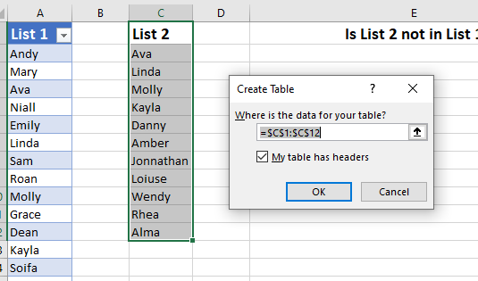
Tables – Comparing lists in Excel where the ranges sizes might change
In each of the formulas we have looked at so far, we have selected a range of cells in our Match functions that is not dynamic. That means if we add new data to one of the lists, we have a manual step to update our formula to include the new data.
To convert the lists to tables, select one of the lists and press CTRL. This is the keyboard shortcut to convert to a table. If you selected the header in the range of cells, ensure you tick the box to confirm your table has headers.
Tables by their nature use structured naming. Therefore, when you are writing a formula and you select a column from a table, it will not show cell references, but the column name.
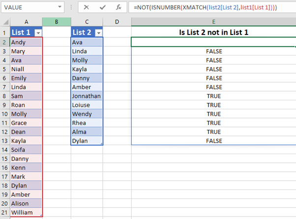
Looking at our previous formula using XMATCH to find items in list 2 not in list 1, we can re-write this function now using our table references
=NOT (ISNUMBER(XMATCH(list2[List 2],list1[List 1])))
Now, as we have used tables, if we add a new row to either of the tables, our spill range will also increase to include the new data.
Highlight differences in Lists using Custom Conditional Formatting
Earlier in this article we looked at a very quick way of comparing these two lists using a predefined rule for duplicates. We can however also use Custom Conditional Formatting. If you are not familiar with Custom Conditional Formatting, I would suggest you check out this article: Excel Dynamic Conditional Formatting Tricks:
We need to look at two different approaches here to highlighting differences. When we are not using tables and we have created a true/false formula to identify the differences, we can take a copy of the formula and add this to our Custom formatting. However, with Tables we need to force the use of cell references.
Copy formula to Custom Conditional Formatting
Start by taking a copy of the formula. As we have tested the formula in the spreadsheet, we can see that it works before we use it in conditional formatting. This is best practice as very often with relative and absolute cell references it can be difficult to get the formula correct.
Select the cells that you want to apply the custom formatting to. Then from the Home ribbon select the conditional formatting drop down and select New Rule
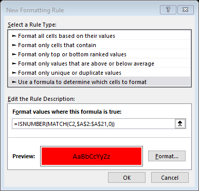
The New Formatting Rule set up box will open and select Use Formula to determine which cells to format. Then paste in the formula and set the formatting type
This will result in all cells that are in both lists being formatted to your chosen format.
Keep in mind that we selected a range of cells to apply this conditional formatting and it is not dynamic. Should we use tables, this would update without the need to change anything!
Other Formulas used to compare two lists in Excel
There are many formulas you can use to compare two lists in Excel. We have already looked at MATCH and XMATCH, but now we are going to look at a few more. Any of the lookup functions will really work along with some others!
VLOOKUP to compare two lists in Excel
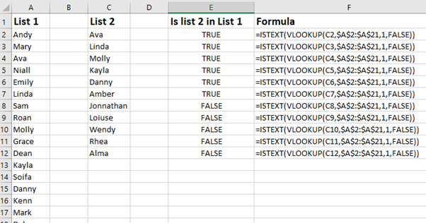
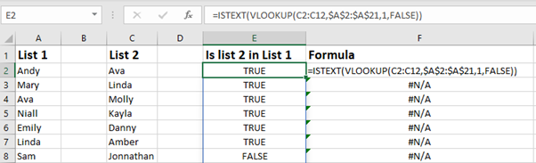
If you are not familiar with VLOOKUP, you can read about it here. Simply put VLOOKUP will return a corresponding value from a cell, if there is no corresponding value an #N/A error will be returned. In our example we are working with text. So, we can carry out a VLOOKUP and test to see if it returns text. If we were using numbers then we could replace ISTEXT with ISNUMBER.
We could use the function =ISTEXT(VLOOKUP(C2, $A$2:$A$21,1,FALSE))
Or if we were using Dynamic arrays in Excel 365, we could use the function
=ISTEXT(VLOOKUP (C2:C12,$A$2:$A$21,1,FALSE))
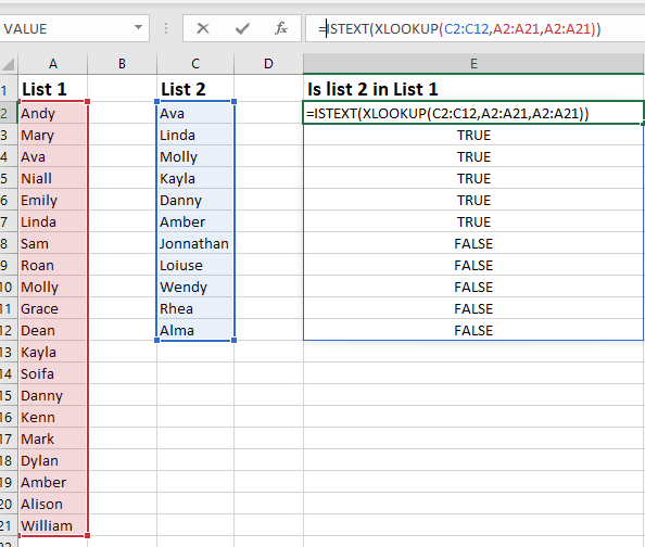
XLOOKUP to compare two lists in Excel
XLOOKUP was introduced in Excel 365 and you can find out more about it here. Very much like VLOOKUP, XLOOKUP will return a corresponding value from a cell, and you can define a result if the value is not found. Using Dynamic arrays, the function would be
=ISTEXT(XLOOKUP (C2:C12,A2:A21,A2:A21))
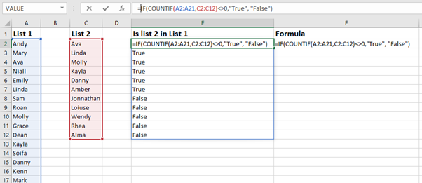
COUNTIF to compare two lists in Excel
The COUNTIF function will count the number of times a value, or text is contained within a range. If the value is not found, 0 is returned. We can combine this with an IF statement to return our true and false values.
=IF(COUNTIF (A2:A21,C2:C12)<>0,"True", "False")
How to compare 2 data sets in Excel
Comparing two lists is easy enough and we have looked now at several ways to do this. But comparing two data sets can be a little more difficult.
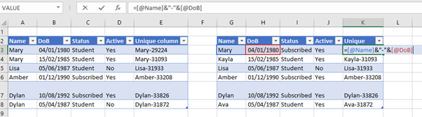
Let us look at an example. We have two tables of data, each containing the same column headers. Looking at the image, we can see matching these two tables would require looking at more than one column.
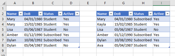
When you need to look at more than one column, the solution would be to create a composite column combining the data into one column. This will create a unique column for each row which we can then use as the matching column
In this example we could combine the Name and DoB to give each table a unique identifier
There are many ways to join contents of a cell, in this case we will do a simple concatenate. As we are using tables, the formula will shoe the table naming format.
Repeat the steps on the second table.
Now we can use any of the examples above to match these two new columns of data. Where they match, we know they match the entire row.
Comparing lists or datasets using Power Query
You can also compare lists and datasets using Excels Power Query. By connecting to the tables and then merging the tables, using different join types we can compare both lists.
In this video you will learn how to compare or reconcile two different data sets using Excels Power query
There is a data set to go along with this video and practice along which you can grab from this article.
However very often you will have datasets where there is no matching column and we need to create a column to carry out a reconciliation between two different lists or two different data sources. In this video you will learn how to create a matching column using power query so you can then compare the data.
SIGN UP FOR OUR NEWSLETTER TODAY – GET EXCEL TIPS TRICKS AND LEARN AND EARN ACTIVITIES TO YOUR INBOX
SIGN UP
Over to you
What way do you like to compare lists or data sets in Excel? Do you use a different option to any of the above? Drop a comment below and you might earn your self some tokens
Don’t have a Hive wallet or a Steempress Account?
I would suggest that you sign up directly for your own hive wallet and sign in to steempress using your wallet. this way all rewards will be paid directly to your wallet within 7 days. You can use this link to sign up now for your Hive wallet
>> GET HIVE WALLET NOW<<
If you sign up using the comments section below you will get a Steempress account. Steempress will hold any rewards you earn until you have a hive wallet.
Have questions? Please use the Hive powered comments section below and we will do our best to help you. Alternatively, you can contact us with this link.
Like what you see? I do hope that you will share this article across your social profiles
Cross posted from my blog with SteemPress : https://theexcelclub.com/ultimate-guide-compare-two-lists-or-datasets-in-excel/
Upvoted by GITPLAIT!
We have a curation trial on Hive.vote. you can earn a passive income by delegating to @gitplait
We share 80 % of the curation rewards with the delegators.
To delegate, use the links or adjust 10HIVE, 20HIVE, 50HIVE, 100HIVE, 200HIVE, 500HIVE, 1,000HIVE, 10,000HIVE, 100,000HIVE
Join the Community and chat with us on Discord let’s solve problems & build together.
I've cross posted it to the Experts Community ☺️