Step by Step - Named Ranges in Excel
(Edited)
Understanding Named Ranges in Excel
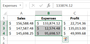
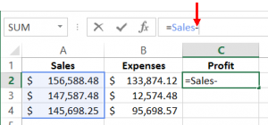
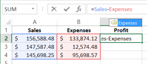
To begin, open workbook 1-1 using Microsoft Excel. Named ranges in Excel are labels that you can assign to individual cells or cell ranges. This allows you to use range names anywhere you would use a cell or cell range reference. For example, you can define the cell range C1:C45 as “Employees.” Now, whenever you need to enter that cell range, you don’t have to remember the exact cell range. You just need to type the name that you used to define it. In addition, range names use absolute cell references. This means if you copy a formula or use AutoFill when working with named ranges, the formula will maintain its original cell reference. Named ranges are most useful when working with formulas as they make them much more readable and improve their overall organization. In the sample workbook, cells A2 and B2 have each been given a name (Sales and Expenses, respectively). Click on cell C2. You can see the formula for that cell displayed in the formula bar: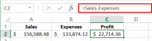
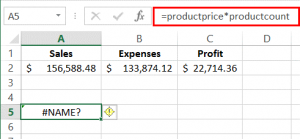
Rather than cell references being used in the formula, there are named ranges. To someone working on this workbook for the first time, this formula is much more self-explanatory than “=A2–B2” would be. Perhaps what is most notable about named ranges is that they allow you to construct formulas before adding the data. When you are designing your worksheet, you can create formulas using names instead of traditional cell references, and then define the names for the corresponding ranges as data becomes available. For example, in the sample worksheet, click to select cell A5. As you can see, this formula (=productprice*productcount) results in a #NAME error. This error will remain visible until both named ranges in the formula have been defined:
Close Microsoft Excel 2013 without saving any changes that you may have made.
Defining Named Ranges in Excel
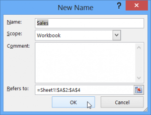
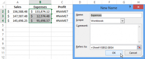
To begin, open workbook 1-2 using Microsoft Excel. To define a range name in Excel, you first need to select the cell or range of cells that you would like to work with. For this example, select cells A2-A4 in the sample workbook. Next, click Formulas → Define Name (not the drop-down arrow):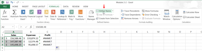
This action will open the New Name dialog box. Here, you can give the new range a name, select which part(s) of your workbook that this range will reference, and add comments. By default, if the cells are all in one row or column, the Name field will be filled in with that column or row’s header (if one has been defined). In this example, you can see that the Sales header has been inserted into the Name field. Leave the default settings unchanged and click OK to apply the new named range:
You will now be returned to the worksheet you’ve been working with. Repeat the above steps to define “Expenses” as the named range for cells B2-B4:
You will now see that the formula that was based upon named ranges has changed to incorporate the values you just defined:
Save the changes that you have made to the current workbook and close Microsoft Excel 2013.
Editing Named Ranges in Excel
To begin, open workbook 1-3 using Microsoft Excel. Once a named range has been defined, you can see the name in the name box (next to the formula bar) when the cell or cell range in question has been selected. For this example, select cells A2-A4. You will see that they have been named “Sales:”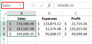
To quickly select a named range in the current workbook, click on the name box arrow and select one of the options listed. For this example, choose Expenses:
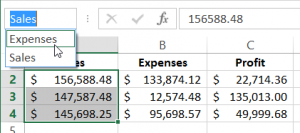
The entire Expenses range is now selected:
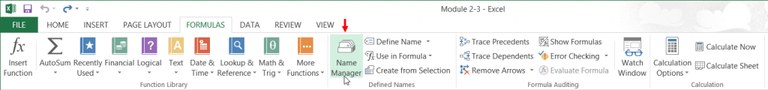
The data within this range may now be modified in any way that you would like. If you insert rows or columns into the range, they will automatically be incorporated. To modify the named ranges themselves, click Formulas → Name Manager:
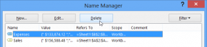
The Name Manager dialog will be displayed. Here, you will see all named ranges inside the current workbook:
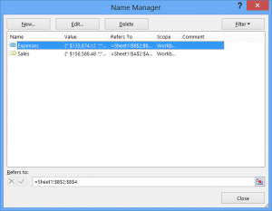
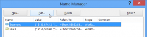
Let’s edit the Expenses range. Click its name to select it and then click Edit:
The Edit Name dialog will now be displayed. Here, you will see controls to change the name, add comments, and change the range of cells:
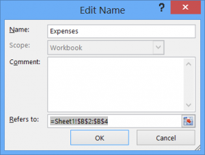
Click Cancel to return to the Name Manager without saving any changes. In the Name Manager, click Close to return to the Excel window. Close Microsoft Excel without saving any changes that you may have made.
Deleting Named Ranges in Excel
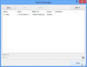
To begin, open workbook 1-4 using Microsoft Excel. To delete a named range, you first need to open the Name Manager. Do this by clicking Formulas → Name Manager: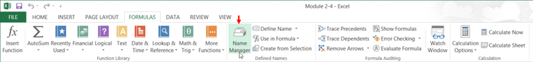
When the Name Manager dialog box opens, you will see all of the named ranges in the current workbook. Delete the Expenses named range by selecting it from the list and then clicking the Delete button:
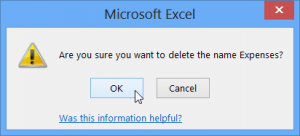
A warning dialog will then be displayed that asks you to confirm the operation. Click OK:
Deleting a named range is a permanent action. You cannot directly recover a named range that you deleted. However, if it was a recent action, it can be undone using the Undo command. You will now be returned to the Name Manager. Here, you will see that the Expenses range has been deleted. Click Close to return to the primary Excel 2013 window:
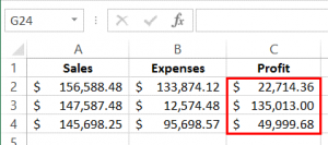
Because the formula in the Profit column uses the Expenses named range, it will now display a #NAME? error. Save the changes that you have made to the current workbook and close Microsoft Excel.
Using Named Ranges in Excel Formulas
To begin, open workbook 1-5 using Microsoft Excel. To use named ranges in formulas, begin with an equals sign like any formula. For this example, select cell C2 and then type an equals sign in the formula bar: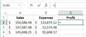
Next, start typing the name of the named range that you would like to use. For this example, start typing “Sales.” A drop-down list will be displayed with a number of suggestions to choose from. Double-click Sales:
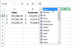
After a named range has been typed into the formula bar, it will be color coded:
Next, you need to add an operator. For this example, type a minus sign (-):
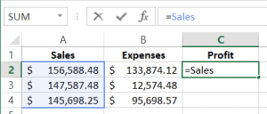
Add the Expenses named range by typing it out fully. Once it is written out entirely, it will also appear color-coded:
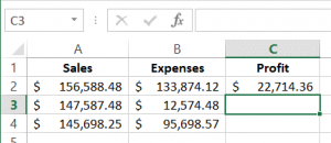
Press Enter to apply the new formula. The results will be displayed immediately:
Save the changes that you have made to the current workbook and close Microsoft Excel.
Take A FREE course with us Today!


Best Value Excel and Excel Power Tool Learning. Access All Areas, Unlimited Learning Subscription

Sign up to my newsletter for Excel and Power BI Tips, Ticks and Hacks
Sign Up
Learn and Earn Activity
-
Now that you have an understanding of Named Ranges, consider the spreadsheets you work with. Describe a workbook and a situation where you could now use Named Ranges? Leave your answer in the comments section below to be eligible for rewards.
-
Have you any questions on Named Ranges, or feedback on this post? If so please use the comments below and you could earn STEEM rewards.

Now there is value in Learning with The Excel Club and our Learn and Earn activities.
Find out more now and start earning while you are learning Excel and Power BI
Cross posted from my blog with SteemPress : https://theexcelclub.com/step-by-step-named-ranges-in-excel/
0
0
0.000
@theexcelclub you made this nice and easy indeed to earn steem rewards. I have a number of spreadsheets set up using named ranges, but most often I would use Table format and use a column name in a formula over a named range. I know you can set up dynamic named ranges, but with tables, if you reference them in a formula and update the table with more data, the formula updates too. with static named ranges this does not happen.
I think I have to make a tutorial on dynamic named ranges now too, tables do rock and that is a great alternative :-)
You got a 60.43% upvote from @bdvoter courtesy of @theexcelclub!
Delegate your SP to us at @bdvoter and earn daily 100% profit share for your delegation & rewards will be distributed automatically daily.
500 SP, 1000 SP, 2500 SP, 5000 SP, 10000 SP.
If you are from Bangladesh and looking for community support, Join BDCommunity Discord Server & If you want to support our service, please set your witness proxy to BDCommunity.
You got a 73.15% upvote from @spydo courtesy of @theexcelclub! We offer 100% Payout and Curation.
Did I say that I love excel.
This is a useful tip and I need to use this more.
Tell us a bit about pulldown menus, functions like sumif (German sumwenn) and the function to color the background by a specific value / range.
Posted using Partiko iOS
hi @detlev - glad to hear you love excel and thank you very much for the suggestions in topics. Stay tuned for more and I will gladly provide tutorials on the same :-)
Named ranges is one of the most useful features that excel has. Before pivot tables and charts, this is one of its core functions that helped me develop and understand excel macros.
A particular scenario I encountered extensive use for named ranges is in a timelogger we use at work.
Particularly, to get a list of deliverables or tasks for a particular development phase like detailed design creation. The excel file we use has a named range "DD" and we use this named range in conjunction with excel's list data validation to be used as a dropdown when inputting a time log. :)
A very helpful topic covered by the @theexcelclub.
Congratulations @theexcelclub!
Your post was mentioned in the Steem Hit Parade in the following category: