---

Warning

Some areas of this post are quite technical in nature. I have deemed this necessary to explain the theoretical structure of a basic intertemporal choice model as well as how it can be adapted to real life decision-making.

---

Hi Everyone,

I have discussed decision-making in several of my posts. These posts have focused on decisions made in the same period. For example, deciding what to eat for lunch or where to go on a day off. Decisions in the present can also effect decisions to be made in the future. Sometimes there is a choice between doing something now or delaying and doing that something in the future. In 2007, I submitted my thesis, ‘Is the pursuit of higher education worth the cost?’. Intertemporal choice analysis was an important part of my thesis. For many, the pursuit of higher education will result in delay of engaging in other activities that require both time and money. I believed an intertemporal choice approach would help me capture a larger share of the opportunity cost than comparing forgone income with the increased income following the completion of a degree.

Basic Intertemporal Choice Model (Irving Fisher Model)

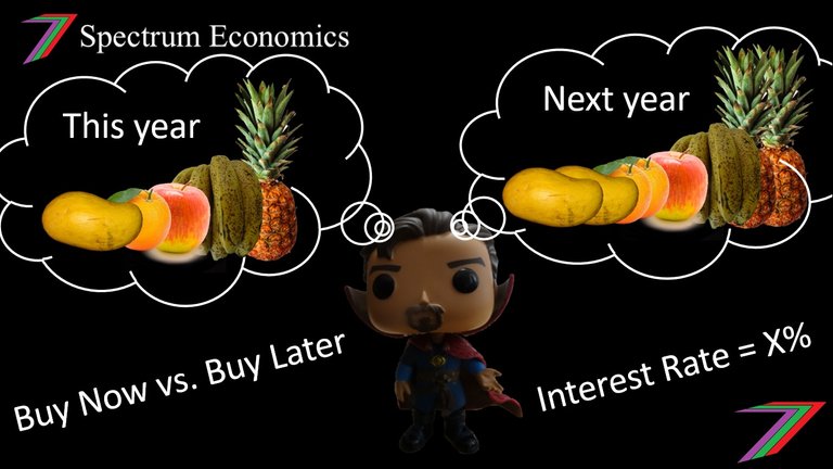
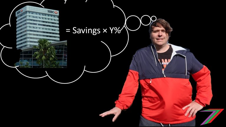
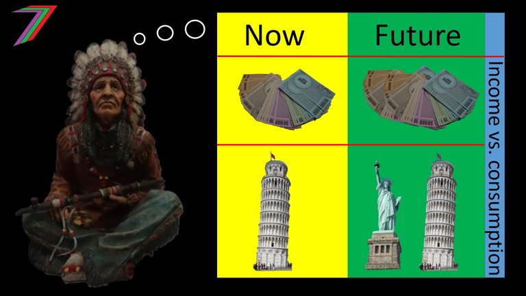
In short, an intertemporal choice model compares consumption choices over different periods. Choices are analysed based on the utility they offer. It is often argued that it is better to have something now than later. However, people have a choice to earn more by delaying consumption. Instead of buying item X today, they could put their money in a savings account or invest it in an asset. With the extra money they earned, they could then buy item X and maybe item Y as well a year later.

Intertemporal choice models often include interest as a return from forgoing consumption. In this post, I will be describing the Irving Fisher intertemporal choice model (sometimes referred to as the Hicks/Marshall model). There are other approaches to intertemporal choice such as the Modigliani’s Life Cycle Hypothesis or Milton Friedman's Permanent Income Hypothesis. However, I believe the Fisher model can be more easily adapted to real world application and therefore the focus of this post.

The model is typically divided into utility functions and constraint functions. The utility function determines the level of satisfaction from consumption in different periods and the constraint function applies the restriction to consumption based on budget/income/wealth. Below is a typical utility function used in an Irving Fisher intertemporal choice model.

Utility = f(C0,C1)
This function can be presented as the following Cobb-Douglas function
Utility = (C0^X)(C1^Y)

Where: C0 is consumption this year, C1 is consumption next year, X and Y are parameters influencing utility from consumption in each year.

Utility functions are assumed to be subject to a budget/income/wealth constraint. This is typically expressed as follows.

Constraint = (1+r)C0+C1=Y1+Y0(1+r)

Where: Y0 is income this year, Y1 is income next year, and r is the real interest rate.

The optimal consumption in each year can be solved using differential calculus and Lagrange Multipliers (λ) as shown below.

U=(C0^X)(C1^Y)-λ((1+r)C0+C1-Y1-Y0(1+r))
δU/δC0=(XC0^(X-1))(C1^Y)-λ(1+r)=0
λ=(XC0^(X-1))(C1^Y)/(1+r)
δU/δC1=(YC0^X)(C1^(Y-1))-λ=0

Substitute λ=(XC0^(X-1))(C1^Y)/(1+r) into (YC0^X)(C1^(Y-1))-λ=0
(YC0^X)(C1^(Y-1))=(XC0^(X-1))(C1^Y)/(1+r)
(XC0^(X-1))(C1^Y)/(YC0^X)(C1^(Y-1))=(1+r)
XC1/YC0=(1+r)
C1=Y(1+r)C0/X – Year 1 Consumption in respect to present consumption
C0=XC1/Y(1+r) – Present Consumption in respect to Year 1 consumption

Substitute C1=Y(1+r)C0/X into (1+r)C0+C1=Y1+Y0(1+r)
(1+r)C0+Y(1+r)C0/X=Y1+Y0(1+r)
C0((1+r)+Y(1+r)/X)=Y1+Y0(1+r)
C0=X(Y1+Y0(1+r))/(X(1+r)+Y(1+r))
C0=X(Y1/(1+r)+Y0)/(X+Y) - Present consumption

Substitute C0=XC1/Y(1+r) into (1+r)C0+C1=Y1+Y0(1+r)
XC1/Y+C1=Y1+Y0(1+r)
C1=Y1+Y0(1+r)/(X+Y/Y)
C1=Y(Y1+Y0(1+r))/(X+Y) - Year 1 consumption

Consumption in each period is dependent upon the parameters X and Y and the interest rate. If the interest rate increases, consumption next year will become more favourable than consumption this year. This can also be demonstrated graphically as shown in Figure 1.

Figure 1: Impact of interest rate on consumption choices

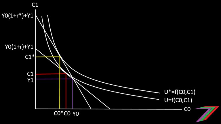
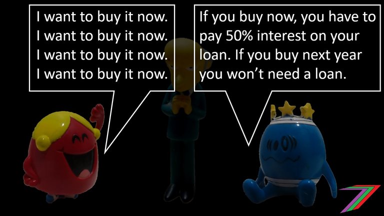
Note: The graph shows that a higher interest rate increases utility. This is only the cases as no pre-existing debt is considered in the analysis.

Parameters X and Y represent the extent of diminishing returns to consumption in each period. The value of X and Y should range between 0 and 1. If X is greater than Y, current consumption is favoured to future consumption.

Example of investment vs consumption

Intertemporal choice models are particularly useful for assessing investment decisions. Investing often involves forgoing present consumption. For example, someone might choose to invest in property and earn revenue from the property by renting it out. The money that went into the investment property could have been used to pay for a holiday and/or luxury items. If the property is a good investment, it will provide a good return and will enable higher expenditure in future periods. A person needs to decide if they are willing to forgo present consumption for a chance for higher consumption in the future.

An intertemporal choice model used to analyse an investment, needs to incorporate risk. This requires a simple adjustment to the existing model. For example, low, high, and medium returns scenarios could be calculated. These scenarios should be assigned probabilities. Risk should be applied to both the income constraint and the utility function.

The income constraint could be presented as follows to determine consumption choices.

Constraint = (1+ρ1rl+ρ2rm+ρ3rh)C0+C1=Y1+Y0(1+ρ1rl+ρ2rm+ρ3rh)

ρ1+ρ2+ρ3=100%

Where: rl is low return, rm is medium return, rh is high return, ρ1 is probability of low return, ρ2 is probability of medium return, and ρ3 is probability of high return.

The utility function can be adjusted as follows to incorporate a parameter for risk (Ψ).

Utility = ((C0^X)(C1^Y))^Ψ

Where:
Risk preferred when Ψ(X+Y)>1
Risk averse when Ψ(X+Y)<1
Risk neutral when Ψ(X+Y)=1

The relative consumption determined using the risk-adjusted constraint could be inserted into the three budget constraints as shown below to determine consumption in dollars.

Income Constraint (low return) = (1+rl)C0+C1=Y1+Y0(1+rl)
Income Constraint (medium return) = (1+rm)C0+C1=Y1+Y0(1+rm)
Income Constraint (high return) = (1+rh)C0+C1=Y1+Y0(1+rh)

Once consumption is determined in each period from each income constraint, they should be inserted into the risk adjusted utility functions. The utility derived for low, medium and high returns should be adjusted based on the probability of each return. The utility derived from the investment option should be compared to utility derived from the almost ‘risk-free’ interest option described earlier in the post.

My contribution to the subject matter

The basic model considers consumption and income for just 2 periods. Such a simple model has limited application to the real world. I intended to use an intertemporal choice model to analyse the decision to pursue higher education. However, I needed to analysis more than 2 periods considering many higher education courses run for more than 3 years and I needed to analyse several years after graduation to analysis the impact of higher education on wages.

A simple extension to the Irving Fisher Model would have been very unrealistic, as the model could analyse the option to spend future income from the degree prior to even starting the degree. I resolved this problem in my model by capping the amount of money someone could borrow in one period. Instead of analysing savings for future periods, I analysed what I called ‘unused liquidity’. Unused liquidity is the sum of the maximum amount that can be borrowed and savings. I assumed unused liquidity would never fall below zero.

The inclusion of ‘unused liquidity’ enabled me to analyse more realistically over 10 periods of future consumption. The analysis could be extended further using the calculated 10 years to establish a trend across a person's working life.

Grounds for applying intertemporal choice to education

Choosing to pursue higher education is an investment in yourself. Therefore, I believe intertemporal choice analysis is a good approach to analysis this decision.

At the end of high school, a person is normally faced with several choices in regards to his or her next journey in life. They could enter the workforce, pursue a degree from a university or learn a trade. These decisions come at a different cost to different individuals. For example, a high performer might receive a scholarship, which reduces tuition fees and other costs.

There are also differences in opportunity costs. The costs of pursuing a higher education might require someone to forgo purchases they could have made if they did not have the costs of education and instead had an income. This cost will be higher for someone who has less wealth. A person with substantial wealth may not need to forgo any purchases. However, even a wealthy person will be required to forgo the time taken to complete the further education.

Opportunity cost can also vary depending on ability. Someone with lower ability might require more time to complete a course, therefore, forgo opportunities for longer. A person may also receive lower grades, which will affect their future income.

Considering that different people have different circumstances, it is logical to analyses different groups of people based on circumstance. In my thesis, I considered wealth, risk aversion, rate of time preferences, ability (grades), gender, age, and life expectancy. The results came back mixed. Pursuing higher education should not always be preferred over an apprenticeship or even directly entering the workforce.

Summary

This post is one of my more technical posts. I feel the technical aspects are necessary to support the usage of intertemporal choice models in analysis. Prior to my Master’s thesis, analysis of investment decisions such as the pursuit of a higher education were analysed based on changes in income. I believed a more relevant analysis should relate to changes in consumption and behaviour. An intertemporal choice model enables me to do that. The Irving Fisher Model was the easiest to adapt for analysis.

More posts

If you want to read any of my other posts, you can click on the links below. These links will lead you to posts containing my collection of works. These posts will be updated frequently.

New Economics Udemy Course

I have launched my first Udemy course ‘Economics is for Everyone’. The course focuses on how economics affects everyday people, the decisions they make and how they interact with the world around them. The course contains 24 video lectures (about 4 hours of viewing), 64 multiple-choice questions (3 at the end of most lectures), 32 downloadable resources (presentation slides, additional notes and links to relevant Steem posts), and 2 scenario questions. The course is currently free-of-charge. Click the link above to access the course.

---

Steem - The Future of DApps