CONSTRUIR LAS ECUACIONES DE UNA RECTA EN EL CONTEXTO DE LA ECONOMÍA. || BUILDING THE EQUATIONS OF A LINE IN THE CONTEXT OF THE ECONOMY.
Conocido el procedimiento para constuir la pendiente de una recta [ Ver post], estamos interesados ahora en construir su ecuación.
Known the procedure to construct the slope of a straight line [See post], we are now interested in constructing its equation.
Ecuaciones de la Recta|Equations of the Line
En todos los textos que tratan este tema conseguirán cuatro tipos de ecuaciones de la recta:|In all the texts that deal with this topic, you will get four types of equations of the line:
Todas ellas llevan a la misma solución: hallar la ecuación de la recta; por ello en este post vamos a tratar el asunto con solo dos de ellas: | All of them lead to the same solution:
find the equation of the line; For this reason, in this post we are going to treat the matter with only two of them:
La ecuación intersección con los ejes coordenados |The intersection equation with the coordinate axes y La ecuación pendiente intersección | The slope intercept equation
Iniciamos con | We start with:
La ecuación Pendiente intersección | Slope intercept equation
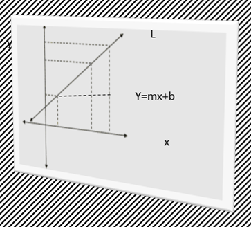
La ecuación Pendiente intersección | Slope intercept equationEsta ecuación tiene dos elementos distintivos: (1) la pendiente m y (2) b (punto de intersección de la recta con el eje de las ordenadas y). | This equation has two distinctive elements: (1) the slope m and (2) b (point of intersection of the line with the y ordinate axis).
Esta es: This is:
y=mx+b
y=mx+bVeamos el siguiente ejemplo: | Let's see the following example
El costo variable de fabricar una mesa es de $7, y los costos fijos son de $150 al día. Determine el costo total y de fabricar x mesas al día. Cuál será el costo de producir 100 sillas?
The variable cost of making a table is $ 7, and the fixed costs are $ 150 a day. Determine the total cost
yof makingxtables per day. What will it cost to produce 100 chairs?
Solución | Solution
Este es un modelo de costo total lineal y viene dado por la suma de los costos variable y fijo Ct= Cv. + Cf. El costo variable depende del número de sillas x que se producen al día lo cual cambia a razón de $7 por día. Esto significa que la pendiente m=7. El costo variable es 0 cuando no existe producción, por lo tanto b=0.
This is a
linear total cost modeland is given by the sum of the variable and fixed costsCt = Cv. + Cf.The variable cost depends on the number of chairsxthat are produced per day, which changes at the rate of$ 7per day. This means that the slopem = 7. The variable cost is 0 when there is no production, thereforeb = 0.
Luego la ecuación de Costo Total es: y=7x+150| Then the Total Cost equation is: y = 7x + 150 .
y=7x+150| Then the Total Cost equation is: y = 7x + 150 .NOTA: Se deja al lector su gráfica y la respuesta a la pregunta formulada en el problema. | NOTE: The reader is left with his graph and the answer to the question asked in the problem
Existe una intersección de la recta P1=(a,0) y P2=(0,b) Pasando La ecuación Que la recta L intersecta al eje de las ordenadas That the line L intersects the ordinate axis Se parte de la ecuación Intersección con los ejes coordenados igualando a We start from the Intersection equation with the coordinate axes equaling Igualamos a Donde En el ejmplo anterior | In the above example Se aplica cuando conocemos dos puntos | It applies when we know two pointsP1=(x1, y1) y P2=(x2, y2) por donde pasa la recta | where the line passes (Supply Equation) At a price of $ 2.50 per unit, a company will offer 8000 T-shirts per month; at $ 4 each, the same company will produce 14,000 T-shirts a month. Determine the supply equation, assuming it is linear. La empresa ofrece 8000 camisetas a 2.50$ y producirá y ofrecerá a 4$, 14000 al mes, por lo tanto la ecuación de oferta dependerá de estos puntos (8000, 2.50) y (14000, 4). The company offers 8000 T-shirts at $ 2.50 and will produce and offer at $ 4.14000 per month, therefore the supply equation will depend on these points (8000, 2.50) and (14000, 4). 2)Usememos el punto (8000, 2.50) [El lector puede usar el otro punto para comprobar que dará el mismo resultado para 2)Let's use the point (8000, 2.50) [The reader can use the other point to check that it will give the same result for Luego la ecuación de oferta es : Then the supply equation is:| Como su nombre lo indica posee dos elementos distintivos: su pendiente In this case, the value of b is calculated using the procedure used in the previous example and then the values of 2 ) Las rectas horizontales tienen pendiente 2 ) The horizontal lines have slope
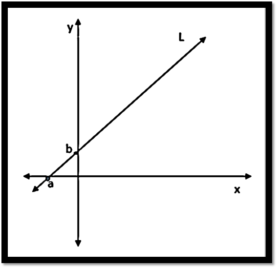
Intersección con los Ejes Coordenados | Intersection with the Coordinate Axes
En la gráfica siguiente: | In the following graph:
L con los ejes coordenados . Tales intersecciones sugieren dos puntos por donde pasa la recta L. | There is an intersection of the line L with the coordinate axes. Such intersections suggest two points through which the line L passes.Ellos son: | They are:
Conocidos esos puntos se calcula la pendiente: | Once these points are known, the slope is calculated:
m=b/-a=-b/a(1)Sustituyendo (1) en la ecuación Pendiente Intersección y=mx+b, se tiene:
y=(-b/a)x +b | Substituting (1) in the equation Slope Intersection y = mx + b, we have:
y = (- b / a) x + b
Trasladando b al miembro izquierdo de la igualdad nos queda: | Moving b to the left side of the equality we have:
y-b=(-b/a)xa como factor al miembro izquierdo, resulta: | Passing a as a factor to the left member, it results:
(y-b)a=-bx
Aplicando propiedad distributiva en el miembro izquierdo se tiene: | Applying distributive property in the left member we have:
ay-ab=-bx
Llevando -bx al miembro izquierdo, y -ab al derecho, resulta:
bx +ay=ab
Finalmente, dividiendo en ambos miembros de la ecuación por ab, nos queda: |Finally, dividing both sides of the equation by ab, we are left with:Intersección con los ejes coordenados. |The equation Intersection with coordinate axes.Ejemplo: En la gráfica siguiente: | Example: In the following graph:
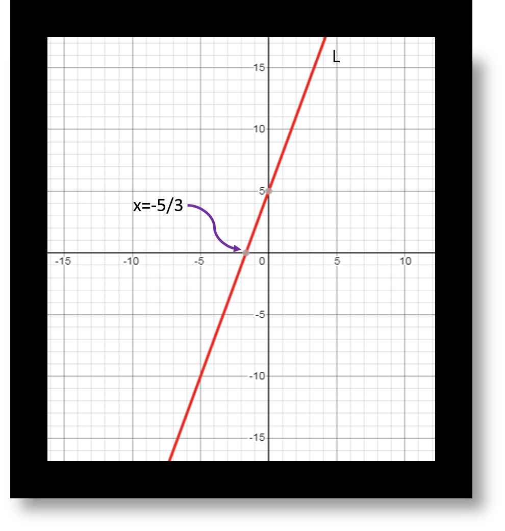
y en b=5, y al eje de las abscisas, en x=-5/3 . Con esta inormación y aplicando (1) podemos obtener su pendiente m.
y at b = 5 , and the abscissa axis, at x = -5 / 3 . With this information and applying (1) we can obtain its slope m``.
Esto es: m=5/(-(-5/3))= 5/ (5/3)=15/5=3. Luego
m=3. | This is: m = 5 / (- (- 5/3)) = 5 / (5/3) = 15/5 = 3. Then m = 3.Por lo tanto la ecuación pendiente inersepción de la recta L, es: | Therefore the slope equation inersection of the line L, is:
y=3x+5
Ecuación General de la Recta |General equation for a straight line0 y eliminando el denominador, así:
0 and eliminating the denominator, like this:
x/a + y/b=10 | We equate to 0
x/a + y/b -1=0
Multiplicando cada término de la ecuación por ab, nos resulta: | Multiplying each term of the equation by ab , we get:a y b son dos numeros reales, distintos de 0, cualesquiera. | Where a and b are two real numbers, different from 0, whatever.y=3x+5, su ecuación general es: | its general equation is:-3x +y -5=0Ecuación Dos Puntos | Two Point EquationL.Ilustremos este caso con un ejemplo en el contexto de la economía: | Let's illustrate this case with an example in the context of economics:
Problema | Problem
(Ecuación de Oferta) A un precio de $ 2.50 por unidad, una empresa ofrecerá 8000 camisetas al mes; a $4 cada unidad, la misma empresa producirá 14000 camisetas al mes. Determine la ecuación de oferta, suponiendo que es lineal.
Solución | Solution
Identificción de los datos | Data identification
Estrategia de solución: | Solution strategy:
Ecuación de Oferta del problema:
m=(4-2.50)/(14000-8000)=1.5/6000=0.00025
Teniendo m se puede obtener el valor de b usando cualquiera de los puntos en la ecuación y=mx+b.
Supply Equation of the problem:m = (4-2.50) / (14000-8000) = 1.5 / 6000 = 0.00025
Having m the value of b can be obtained using any of the points in the equation y = mx + b .
b].
Partimos de y=mx+b, sustituimos las coordenadas del punto dado (8000, 2.50) en esa ecuación así: 2.50=(0.00025).(8000) + b
Resolviendo la multiplicación nos queda: 2.50=2 +b.
Despejando b resulta: b=0.50.
b] .
We start from y = mx + b, we substitute the coordinates of the given point (8000, 2.50) in that equation like this: 2.50 = (0.00025). (8000) + b
Solving the multiplication we have: 2.50 = 2 + b.
Solving for b results in: b = 0.50 .
Solución | Solution
y=0.00025x + 0.50
La gráfica se deja al lector.| The graph is left to the reader.
#Finalmente
La ecuación Pendiente intersección. | Slope intercept equation.m y un punto | As its name indicates, it has two distinctive elements: its slope m and a point P=(x1, y2).En este caso se calcula el valor de b usando el procedimiento utilizado en el ejemplo anterior y luego se sustituyen los valores de
m y b en la ecuación y=mx +b obteniéndose así la ecuación deseada.
m and b are substituted in the equation y = mx + b , thus obtaining the desired equation.
Observaciones: | Observations:
x=a.
x = a.
0, por lo tanto si sustituimos este valor en cualquiera de las ecuaciones anteriores, nos resulta que: y=b, es decir, su ecuación queda definida por su intersección con el eje de las ordenadas.
0, therefore if we substitute this value in any of the previous equations, we find that: y = b, that is, its equation is defined by its intersection with the ordinate axis.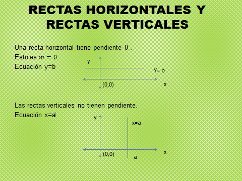
Referencia|Reference
Matemáticas aplicadas a la administración y a la economía. Jagdishh C. Arya/ Robin W. Lardner. Tercera edición. | Mathematics applied to administration and economics . Jagdishh C. Arya / Robin W. Lardner. Third edition.
Créditos./Credits
El contenido de este post es totalmente inédito y se ha elaborado con ayuda de las herramientas electrónicas Excel y PowerPoint./The content of this post is totally unpublished and has been prepared with the help of the electronic tools Excel and PowerPoint.