Citizen science: Top quark production at CERN's Large Hadron Collider
There were so many things that have happened last week. Even though I was able to work on the fourth set of tasks for this project, I had to put aside the writing part of my progress since I had to spend my weekend for some urgent work tasks. Last week was also the end of summer season in our country, we're now in the season when every afternoon heavy rain pours. The drastic transition from hot and humid to cold and rainy days was so evident that my body take its toll 😩 which further delay my writing.
I was actually very excited when I was trying to understand what the histograms show because it was also last week when I was able to finish reading one of the published article related to this project. I thought about how some of the figures in the article are similar in form with the results we are able to produce in this set of tasks. I had a feeling of wearing a particle physicist's hat for a few seconds, hahaha.
And now, before I discuss about this week's progress. Here's just a quick review of how far we've come already in this project, that you may take interest and hopefully join us:
- Installation of the tools [MG5aMC] necessary for particle physics simulation
- Using the MG5aMC to simulate top quark production at CERN's LHC
- Installation and use of MadAnalysis 5 for detector simulation and event reconstruction
For the set of tasks this week, we investigated the simulated collisions and studied their properties in the same way a with the particle physicists, which explains what I felt in my story. ☺️ To follow on this progress report, you can check on the fourth blog post of the citizen science project by @lemouth, Citizen science on Hive - Deciphering top quark production at CERN's Large Hadron Collider.
From the previous set of tasks, where we performed event reconstruction on the simulated collisions, we use those to analyze the resulting higher-level objects which are the electrons, muons, taus, jets, photons, and missing energy. We start by launching MadAnalysis5 in the terminal by typing
./bin/ma5 in the directory named madanalysis5.Next, is we import the simulated events once the prompt >ma5 shows in the terminal:
ma5> import ANALYSIS_0/Output/SAF/_defaultset/lheEvents0_0/myevents.lhe.gz as ttbar
And then, we set the production cross section associated with this event sample to 505.491 pb by typing
ma5> set ttbar.xsection = 505.491. As I remember, I got a different production cross section from the samples I've simulated. It was mentioned in the tutorial post that I can use this value instead, I wonder though, how does this affect the analysis?Normalization of the reconstructed events
The first thing to do before we proceed on the analysis is to normalize the reconstructed events in terms of high-level objects to the amount of collisions recorded during the full run 2 of the LHC. We do this my indicating in the MadAnalysis5 the value of the luminosity to 140fb-1. The luminosity is defined as the measure of how many particles can be squeeze through a given space in a given time which does not necessarily mean that the particles collide.
ma5> set main.lumi = 140
ma5> plot NAPID
ma5> submit
ma5> open
This will give us the results shown in Figure 1 where the y-axis indicates the value of luminosity we used. The histogram shows the distribution of our reconstructed events where we can see a lot of b-jets (b~/b column), some electrons (e+/e- column), some missing energy (ve~/ve column), some muons (mu+/mu- column), really a lot of jets (g column), and a bunch of photons (a column).
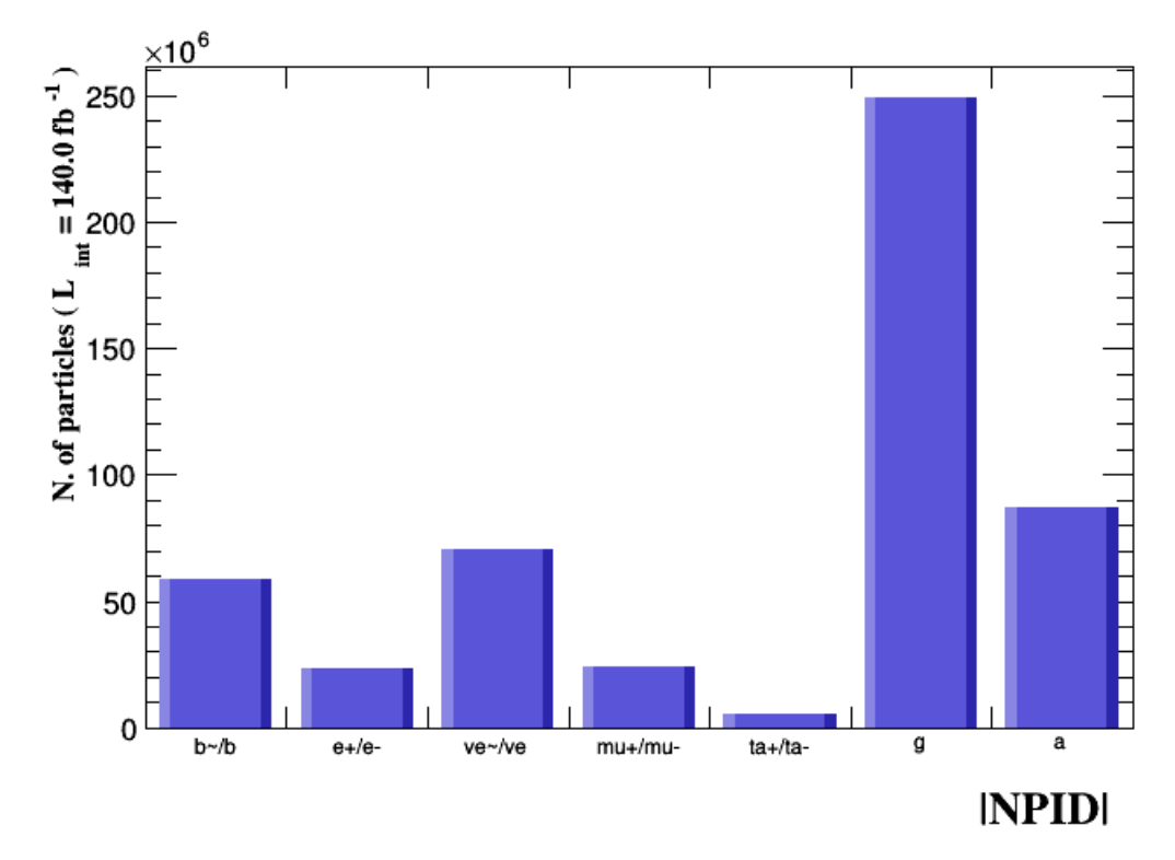
The distribution is very reasonable as it agrees with what actually happens in the LHC. To explain further, a top-antitop pair decays immediately and produces a b-quark and a W boson. A b-quark gives rise to a b-jet which corresponds to a jet of strongly-interacting particles. There are two b-jets produced in every single simulated collision, one from each of the decay of the top quark and top antiquark. The identification of the b-flavour of the jets is not a 100% efficient process, some are identifies as light (i.e. normal) jets which contributes to the column g in Figure 1.
In the same manner with the b-jets, there are two W bosons that originate from the top quark and top antiquark. The instantaneous decay of a W boson produces either of the following:
- one electron and one neutrino
- one muon and one neutrino
- a pair of light jets
- one tau lepton and one neutrino
The decays occur at the same rate except for the option where a pair of light jets is produced, which is more frequent. The large amount of light jets for this reconstructed events can be attributed to the mistagging of the b-jets, more frequent decay rate from the W bosons, and lastly, from radiation. The questions that come to mind are quite general, what are the factors that affect the reconstruction to higher-level objects? (especially for the case of taus). And, are these factors also the reason for the efficiency problem of identifying the b-flavour jets as mentioned earlier?
Particle multiplicity
The amount of light jets and photons observed in the event final state comes from the very energetic particles which radiate a lot. However, some of these radiations are often not so energetic. In order to focus on the objects that have sufficient energy, an additional step to our analysis is to 'clean' our sample set. For the series of particles in this set of tasks, we have imposed values of transverse momentum that will be ignored.
Lepton multiplicity
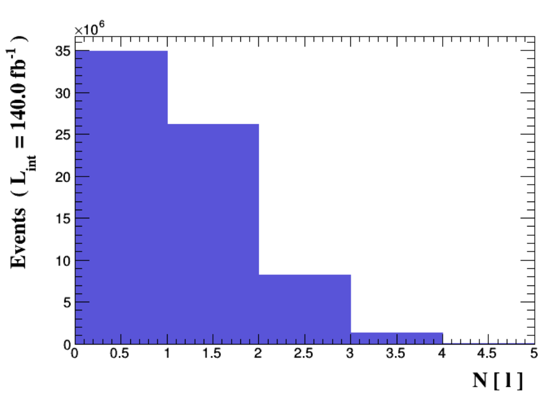
The leptons are the electrons, muons, taus, neutrinos, and their corresponding antiparticles. We implement a cut on the leptons with PT < 20 GeV using the following commands:
ma5> define l = l+ l-
ma5> plot N(l) 5 0 5
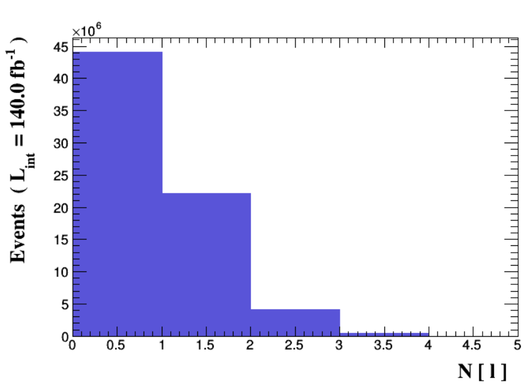
ma5> select (l) PT > 20
ma5> plot N(l) 5 0 5
ma5> plot NAPID
ma5> resubmit
ma5> open
In the code, we define the leptons (l) in the way that the program understands. The values 5 0 5 in the plot command means that there are 5 bins ranging from 0 to 5. The N sysmbol indicates that we want to determine the multiplicity of the particles in some object. The resulting histograms are shown in Figure 2.
Photon multiplicity
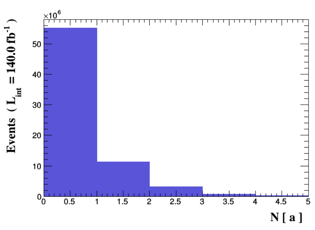
We impose the same cut restriction for the photons using the same commands, only we change the symbol from
l to a, which is the label that corresponds to photons in MadAnalysis5. Figure 3 shows the resulting histograms for the multiplicity of the photons.It was mentioned from the tutorial that a general trend of a migration of events from the right part to the left can be observed upon imposing the cut. This is because the not so energetic charged particles are ignored, thus their number decreases. This effect is obvious in the zero-bin photons in the histogram after the cut (in Figure 3) which shows the removal of most photons that originate from radiation.

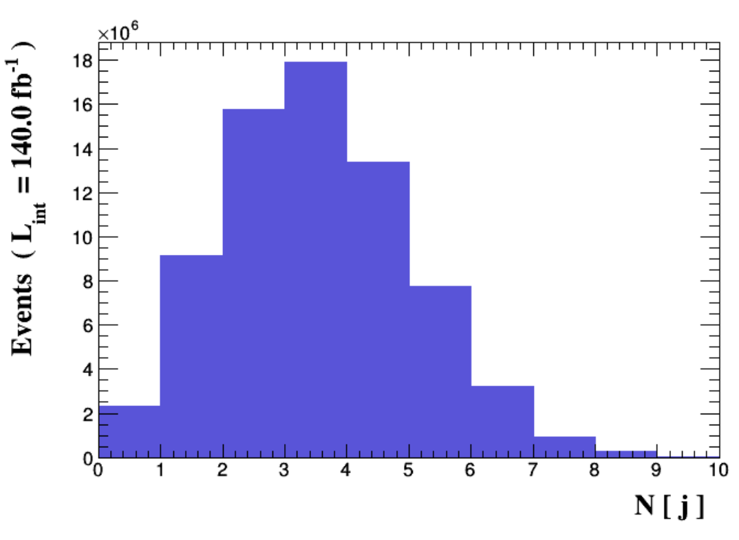
Jet multiplicity
Here comes the first of the tasks we did independently from the tutorial, haha, it is to redo the selection cut for the b-jets. Using the same commands, I used the label
j and imposed a selection cut where we ignore the jets with PT < 25 GeV. The resulting histogram in Figure 4 shows that the migration shifted from left to right. The b-jets with higher multiplicity remained after the imposed selection. My guess comes from what I remember from the introduction to particle physics course I took online years ago, that jets have large transverse momentum that is also why they can reach the outer layer of the detector which measures the hadronic decays. By considering objects with higher values of transverse momentum, we observe showers with higher multiplicity of jets in the distribution. 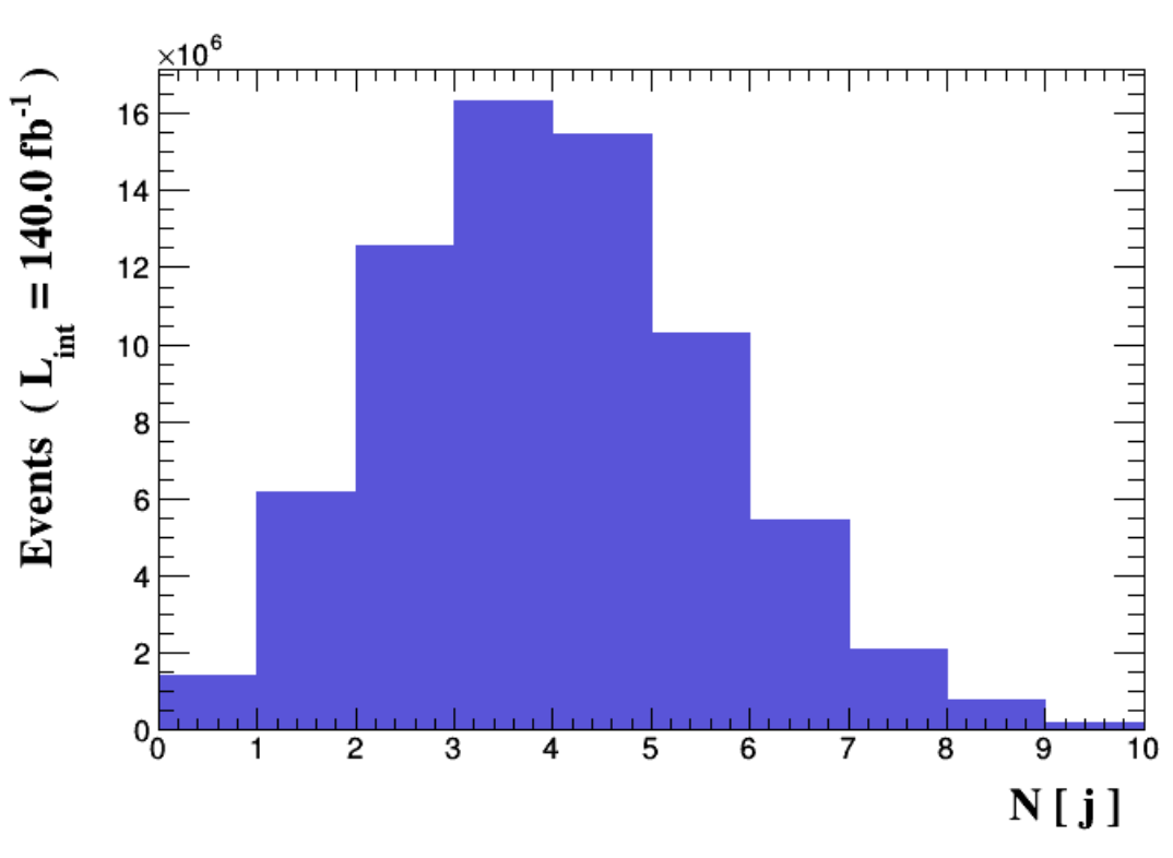
Selection of a subset of all simulated collisions
In this section, we select a subset of all generated collisions to study the properties the object of our concern. In this example, we enforced one of the top quarks to decay into one lepton, one neutrino, and one b-jet. The other top quark will then be enforced to decay into one b-jet and two light jets. The subset we focus on is the event final state that consists of exactly one lepton. To do this, we use the command:
ma5> select N(l) == 1. This cut as shown in Figure 5 has an efficiency of about 30%, which means that about 30% of all events feature exactly one lepton in the final state.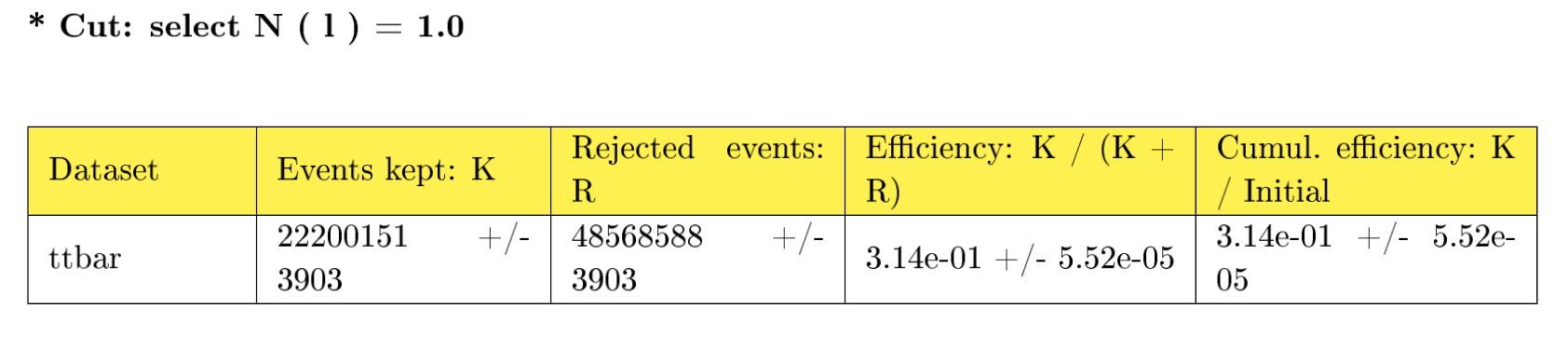
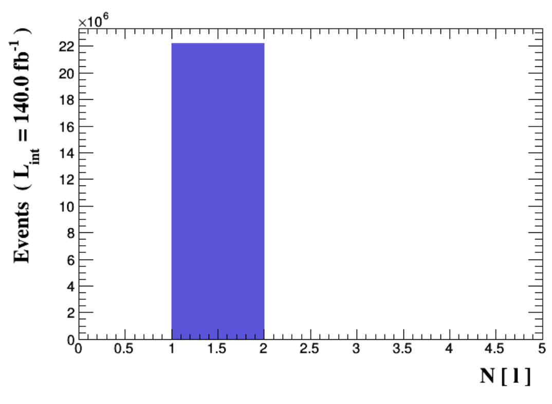
Again, looking into the multiplicty distribution of the leptons after the imposed cut. The resulting histogram in Figure 6 shows that there are only one lepton (one-bin lepton) event final state in the subset.
The properties of a lepton
The particles of objects in our event can be distinguished from their properties. The transverse momentum is one of them, the other one is the pseudo-rapidity that indicates how central an object is in a detector. An object is very central to the detector if it has a small pseudo-rapidity values and longitudinal if large.
To observe the values of these lepton properties, we look into their distribution. In MadAnalysis 5, we type the following commands:
ma5> plot PT(l) 25 0 200 [logY]
ma5> plot ABSETA(l) 25 0 2.5 [logY]
ma5> resubmit
ma5> open
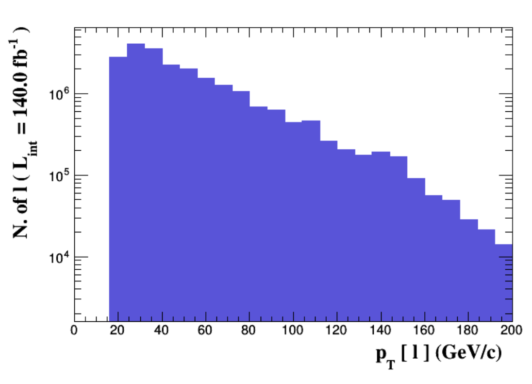
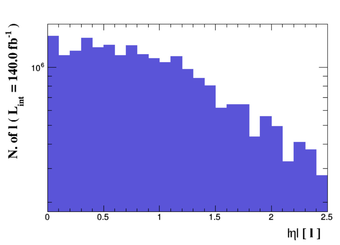
Comparing the results shown in Figure 7 from the histograms in the tutorial, I noticed a difference in the distribution of the pseudo-rapidity. The one from the tutorial looks more uniform compared to the results I've got. I wonder what could be the reason for this?
The mass of a W boson
Another thing we can investigate on is the mass of the combination of jets in the selected events. Since the two top quarks are enforced to decay and produce two b-jets. We mentally combine the two jets and observe the resulting distribution. To do this, we type the following commands:
ma5> plot M(j[1] j[2]) 50 0 250 [logY]
ma5> resubmit
ma5> open
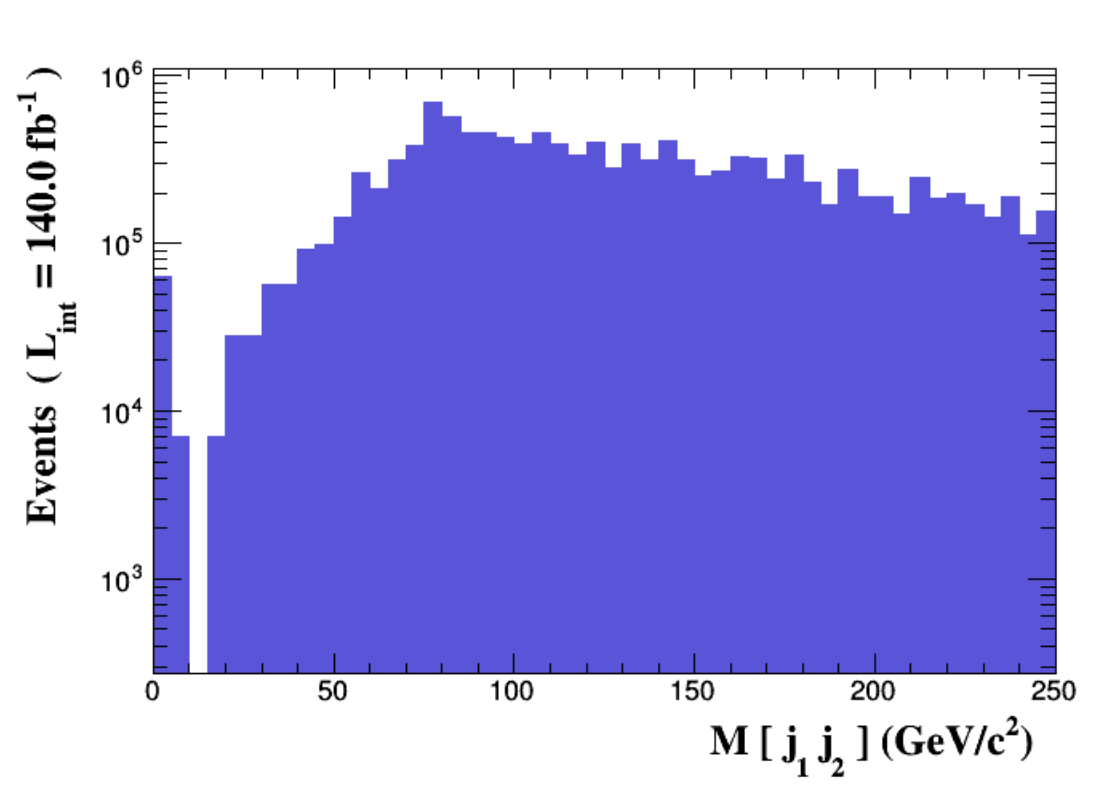
The resulting histogram in Figure 8 shows a peak around 80 GeV which corresponds to the mass of the W boson. As mentioned previously, the two jets we combined have an intermediate W boson in the decay. Amazingly, this is how particle physicists look for the presence of real intermediate particles in a process. It is to try to reconstruct peaks that appear in the middle of distributions. What an experience to be able to do the same work! :)
Missing transverse energy spectrum
Here's the last task we have to work on independently, I must say, the questions accompanying the homework were really helpful. I was obliged to think make sense the results I got, not in a way that I should get the right answers only. The questions were like fuel to my curiosity that I had to answer the whys in the hope that it does make sense hahaha. To generate the missing transverse energy distribution, we use the following commands:
ma5> plot MET 50 0 500 [logY]
ma5> resubmit
ma5> open
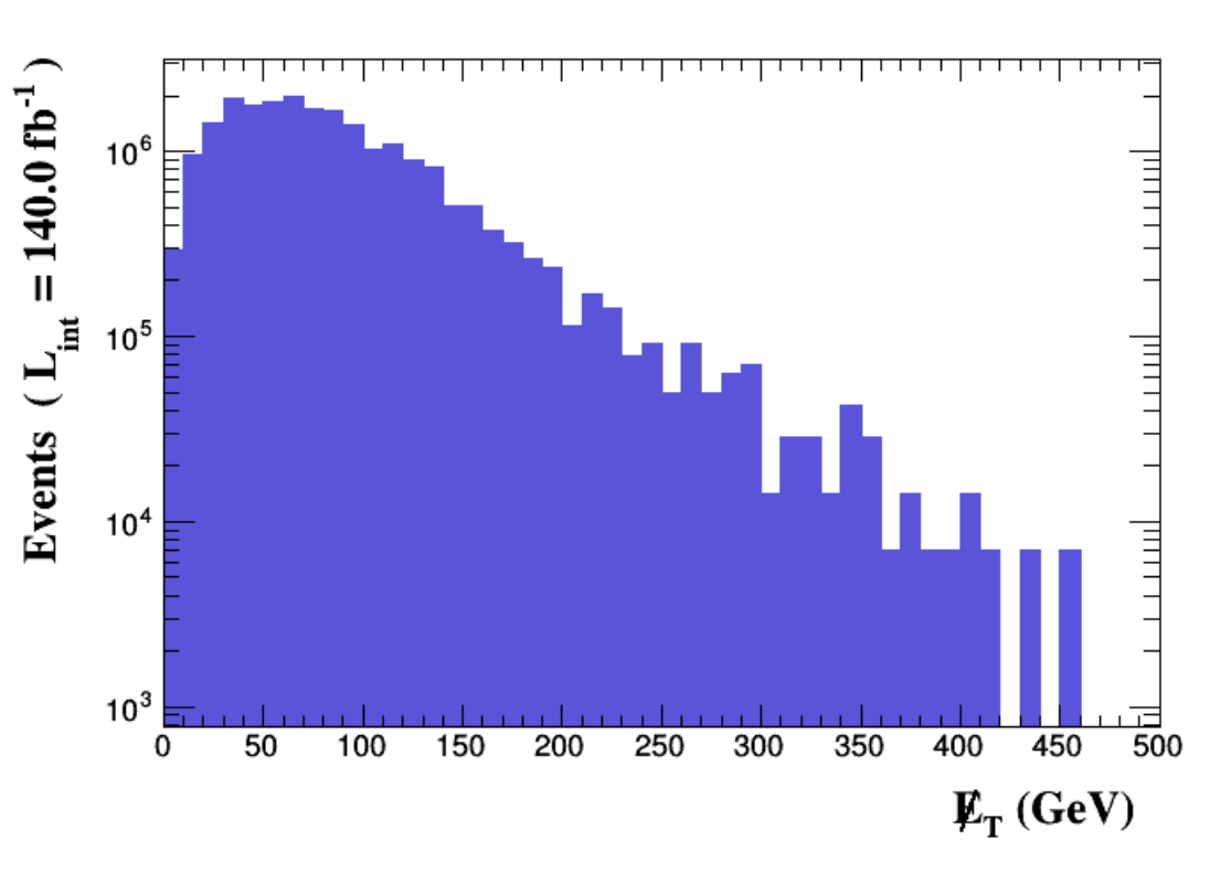
I have chosen a wide range of values to consider for the reason that I may see the bigger picture. Haha. The histogram in Figure 9 shows a distribution skewed to the left or the low-value transverse momentum. This could be the reason why the missing energy is difficult to measure since bulk of these missing energies have low level of energy.
Links of my progress reports for this project:
0
0
0.000
i did not understand a thing. lol.
Hahaha. It would be helpful to read on the blog posts of lemouth. 😀
This is so comprehensive. Good work. Our prof will soon be here to grade you :) @lemouth
[x] Done ^^
Thank you for that remark :)
Great Post!
!1UP
Thank you for the support! :)
You have received a 1UP from @luizeba!
@stem-curator, @vyb-curator, @pob-curator, @neoxag-curatorAnd they will bring !PIZZA 🍕
Learn more about our delegation service to earn daily rewards. Join the family on Discord.
Thanks for your contribution to the STEMsocial community. Feel free to join us on discord to get to know the rest of us!
Please consider delegating to the @stemsocial account (85% of the curation rewards are returned).
You may also include @stemsocial as a beneficiary of the rewards of this post to get a stronger support.
I hope you have recovered health-wise, and that your urgent work-related tasks did not disturb your life too much and are now resolved. On my side, I am happy to finally got the possibility to read your report, and I am even happier to discover that you had read my PRD paper of last year. In one of the next tasks, we will try to reproduce some of the figures in this article (those from section V).
Let me now go through your report, answer your questions, and comment your findings. Feel free to come back to me if necessary.
When we calculate those cross sections, of course there is an uncertainty attached to them. First of all, we have a purely numerical uncertainty as we used a numerical method to compute a complicated integral. Second, there is a theory uncertainty inherent to how quantum field theory functions. Therefore, even if your value is slightly different from mine (it should however be similar), this is not a big issue. At the end of the day, we will have to deal with uncertainties, but that’s too early for that, especially as MadAnalysis5 cannot account for them yet (this is a project we currently have within the Google Summer of Code 2022 session).
For what concerns b-jet identification, we rely on the fact that after hadronisation (formation of composite particles made of quarks and antiquarks by virtue of the strong force), hadrons decay into each other and form jets. For hadrons originating from a b-quark, named B-hadrons, they fly a bit in the detector before decaying. This gives measurable displaced vertices. However, observing the displacement is imperfect, and this contributes to the mistagging rate. The exact details of the identification process depend on hadron and jet properties (their energy, momentum, etc.), but I hope the above gives you the idea.
For what concerns tau, the situation is a bit different. Tau leptons sometimes decay into muons and electrons (and neutrinos that run away as missing energy). In this case, we have what we call a leptonic tau. This happens in roughly 35% of the time and there is very little hope to reconstruct the tau as much of the information is gone. In 65% of the case, the taus decay into jets and neutrinos (again, missing energy). Those jets have however special properties (they contain very few charged particles, are narrow, etc.) so that we have handles to identify the initial tau. As this is imperfect, many taus will be lost in the process.
Please don’t hesitate to come back to me if needed.
In fact, in the code by default taus are not considered as leptons. Strictly speaking, they are of course leptons. However, they will always decay either to jets (in this case they can be identified as taus with a decent efficiency; see above) or electrons/muons. Therefore, when we say leptons, taus are excluded (because they are special).
Here, the discussion should be restricted only to b-jets and not all jets. In the case of b-jets, it is true that they have a higher transverse momentum (in average), which is why they are mostly agnostic on the cut. Now the next question is why they have such a large transverse momentum. Do you have an idea?
I am not sure to follow you on the above statement. Do you mind clarifying what you meant? Thanks in advance.
I do not think it is the case. Please check the Y-axis range. This is where we have a difference.
In the Standard Model, the only source of missing energy consists of neutrinos, and they always come from W boson decays into a lepton and a neutrino. Therefore, those neutrinos usually get half of the W boson mass, which is why we have a peak around 40-50 GeV. That’s the most frequent outcome.
Cheers, and thanks again for your hard work! This report was amazing! You managed to get all questions of the assignments right.
Wow, I'm looking forward on this one! I also have some questions I noted while reading the paper that I'd like to look more into or maybe ask you of when I'm done reading it through again, hope that's okay with you. :)
Is this what happens in the detector during experiments?
It is always OK to ask questions :)
Yes. We can really "see" the displacement as recorded by the electronics. See for instance this image. The dashed lines are associated with neutral objects and leave no tracks in the most central part of the detector. We thus have a bunch of displaced phenomena.
In fact, this is not exactly the good answer. A very massive particles could have a small transverse momentum, and vice versa. You have to think about where the b-jet is coming from. This will probably help you to find the answer.
Could be. We have showers of quarks and gluons (quarks and gluons radiating quarks and gluons radiating quarks and gluons, and so on). Then all final state particles hadronise, decay in other hadrons and so on. We finally reconstruct jets from there. How many jets we end up with depends on the initial process (as most radiation and hadronisation sub-processes are collinear). I hope this will help you (I am still very unsure to understand what you meant... :D ).
I still think it is an artifact of the figure. Maybe by checking carefully (with the same y-axis), they will look the same. I assume you have used root for the plots. If you know how to handle root files, I can tell you how to modify them to change the axis range.
Cheers!
At this point, I think it'll pay off if I review on the materials of that introductory course. :) Especially on the things you have pointed out.
Regarding with the plot, ma5 does use root, I didn't change it before since I was able to reproduce the histogram we first generated. Also, I didn't have an idea how to do it. What you mean with modifying root files is accessing the root file system of ma5? If it is, I think I'll be able to modify the axis range given your instructions on what files I have to access. :)
You can change the default plotter used in MA5 as follows, if you have both ROOT and MatPlotLib installed. Once the program is started, please just type:
(or= root).The plots I generated are obtained with matplotlib, and this may explain sometimes a different behaviour.
As another possibility, you can go to the
ANALYSIS_1/Output/Histos/MadAnalysis5job_0folder (please adapt the name of the first subfolder to that relevant to your case). You got the root files associated with each associated histogram.You can modify them (to enforce a particular Y-axis range in) and run them again to generate modified histograms. You also have the matplotlib files in Python and can work from these.
I hope this helps!
Cheers!
Dear @travelingmercies, we need your help!
The Hivebuzz proposal already got important support from the community. However, it lost its funding a few days ago and only needs a few more HP to get funded again.
May we ask you to support it so our team can continue its work this year?
You can do it on Peakd, ecency, Hive.blog or using HiveSigner.
https://peakd.com/me/proposals/199
Your support would be really helpful and you could make a difference.
Thank you!