Master Pivot Tables with these 8 How-to Tricks
Pivot Tables are a core tool in Excel used to quickly analyze large, or small, sets of data. Yet many Excel users have a fear of Pivot Tables as they are often viewed as a more advanced tool. I would argue Pivot Tables are a core feature, that every Excel user should know.
In this article, we will explore 8 How-to tricks when working with Pivot Tables
Master Pivot Tables with these 8 How-to Tricks
How to turn on or off the Pivot Table field list
When you select a Pivot Table, by default the Pivot Table fields list should be on the right side of your screen. However, this often gets turned off.
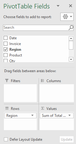
To turn on, or off the Pivot Table fields list, click on the Pivot Table and select the Pivot Table analyze tab on the ribbons. Under the Show group of commands, select Field List. This will allow you to toggle on or off the fields list.

How to expand or contract fields
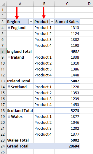
Very often Pivot Tables contain more than one field in the Rows. This gives rise to a hierarchy. And the ability to expand and contract the views of these hierarchies on the Pivot Table. In the example shown, Region is the first field on this Pivot Table and Product is second. On the Pivot Table, we have these little expand or collapse buttons.
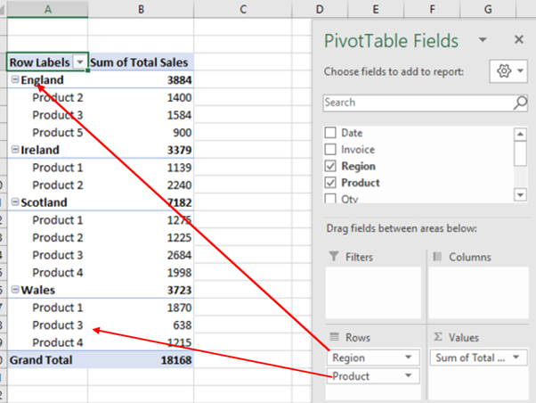
I have seen many Excel users manually expand and contract each level on a Pivot Table, unknown to them there is a quicker way to achieve this.
On the Pivot Table Analyse tab of the ribbons, under the Active Field set of commands, you will find the options to Expand or Collapse Fields.

When all the fields of a Pivot Table are expanded, by selecting the first cell with the collapse button on the Pivot Table, and select Collapse Field from the ribbon, all of the Pivot Table will collapse.
If you select a lower hierarchy and select collapse from the ribbon, only that hierarchy and those below will collapse.
How to name a Pivot Tables
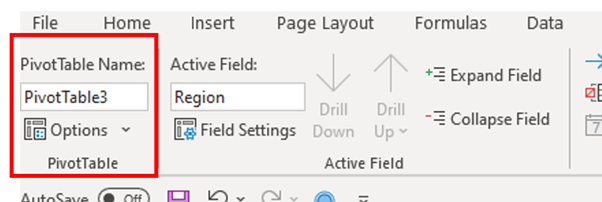
Naming Pivot Tables is a useful habit to get into. When you are working with multiple Pivot Tables in one workbook, naming really comes in handy.
The naming box can be found on the far left of the Pivot Table analyze tab. Select the Pivot Table you want to name and in the name box, type in the name. There are a few limitations to this. You can not use duplicate names on the same sheet. You can also not use any special characters in the name.
How to add or removed totals and subtotals from your Pivot Table
Totals and subtotals can be added and removed from a Pivot Table allowing you more customization over how it looks.
From the Design tab of the ribbons, select Grand totals. This will give you the options to turn on and off the Grand totals on a Pivot Table.
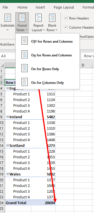
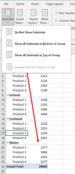
You can also turn on and off the subtotals. From the Design tab of the ribbons select Subtotals. Options include Do not show subtotals, Show subtotals at the bottom of the group and show subtotals at the top of the group.
How to change the layout to a tables style format
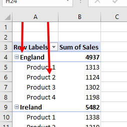
The standard layout of a Pivot Table is known as compact form. This is where all fields placed in the rows of a Pivot Table show up in the same column in the Pivot Table. As we can see from the Pivot Table, both Region and Product are showing in Column A.
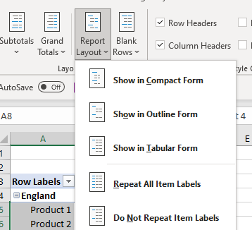
From the Pivot Table design tab, the Report Layout option allows Excel users to change this.
By selecting Outline Form, the second and subsequent fields of the rows in the Pivot Table will move to the next available column in Excel.
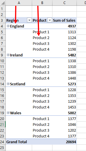
By selecting tabular form we will see a similar indent of the fields to new columns, however, the subtotals move to the bottom and the Pivot Table has a different look and feel.
How to change the aggregation type on the values fields to Average or Count
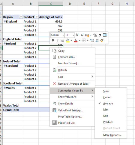
The default aggregation type on Pivot Tables for numerical data is SUM. For categorical data it is COUNT. By selecting a field on the Pivot Table, right-clicking, and selecting Summarize value by, you are given the option to change the aggregation type. From here you have the option to select COUNT or AVERAGE along with other functions.
How to show values as a % of total
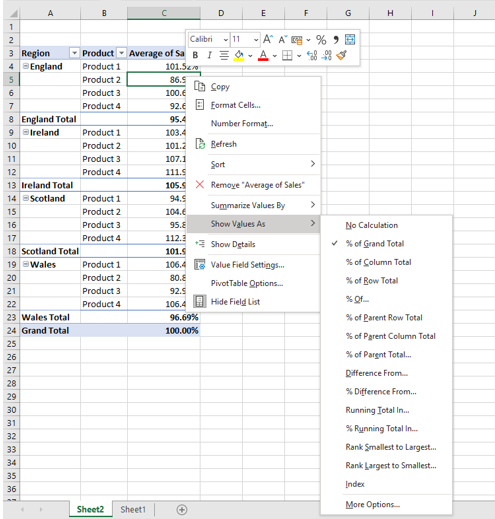
In addition to changing the aggregation type, when you are using Pivot Tables you can also quickly change how the value is shown. For example, you can choose to show the value as % of Grand total and you also have many other quick calculations available.
How to change the value of errors, or blanks to a value of your choice.
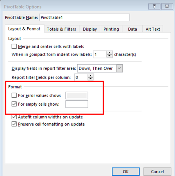
When working with Pivot Tables you may have the need to define values for errors or empty cells. To do this, right-click on the Pivot Table and select Pivot Table options. On the first tab of the Pivot Table options box, Layout & Format, under the Format option, users can define values for errors and empty cells.
Take A FREE course with us Today!

- includes XLOOKUP and will soon include Dynamic Arrays

Power Query Excel 365

Best Value Excel and Excel Power Tool Learning. Access All Areas, Unlimited Learning Subscription

SIGN UP

- includes XLOOKUP and will soon include Dynamic Arrays

Power Query Excel 365

SIGN UP
I would suggest that you sign up directly for your own hive wallet and use this to sign into the comments below. This way all rewards will be paid directly to your wallet within 7 days. You can use this link to sign up now for your Hive wallet
>> GET HIVE WALLET NOW<<
Have questions? Please use the Hive powered comments section below and we will do our best to help you. Alternatively, you can contact us with this link.
Like what you see? I do hope that you will share this article across your social profiles


Perfect tutorial on pivot tables, great work, will definately subscribe to your newsletters. Keep up the work you are doing
Congratulations @theexcelclub! You have completed the following achievement on the Hive blockchain and have been rewarded with new badge(s) :
Your next target is to reach 43000 upvotes.
You can view your badges on your board and compare yourself to others in the Ranking
If you no longer want to receive notifications, reply to this comment with the word
STOPCheck out the last post from @hivebuzz: