Signal Processing: Analog-to-Digital Conversion

1. Introduction

Most of the signals encountered in science and engineering are analog. Analog signals are a function of a continuous variable of time or space and have a variable range, which carries information. They naturally occur as audio, image, video, or biological signals. We processed these signals to change their characteristics or extract some desired information by an appropriate analog system. The problem with an analog signal is we need to redesign hardware to tailored fit to a task.

In contrast, digital signals programmable and transferable, which makes them easier to analyze. Digital signal processing is a straight forward task. We convert the analog signal in a sequence of numbers and process by software rather than redesigning a complex circuit. To process the signal digitally, we need an interface that translates the analog signal to the digital processor. The interface is called an analog-to-digital converter. In this blog, we discussed how we mathematical model an analog signal digitally.

2. Analog-to-Digital Conversion

2.1 Sampling

We discretize a continuous-time signal by periodically sampling the signal. A convenient approach in sampling a signal is to multiply an impulse train,

to form the sampled signal,

>

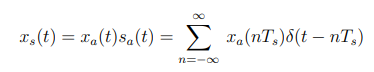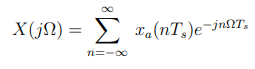
Then, we map the sampled signal into the impulses that are space in Ts (sampling time) into a sequence x(n), where the sample values are indexed by a variable n:

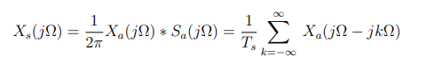
We can analyzed continuous to discrete transformation in frequency domain. Hence the Fourier transform of δ(t − nTs) is e^−jnΩTs, we have the Fourier transform of the sampled signal x_s(t) as

The Fourier transform of the impulse train s_a(t) is given by

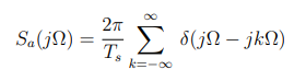
where Ωs = 2π/Ts is the sampling frequency in radians per seconds. Therefore,

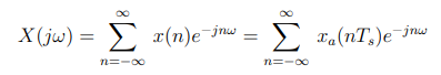
The discrete-time Fourier Transform of x(n) is

A frequency-scaled version of Xs(jΩ) is defined as

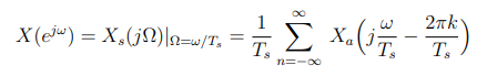
where its scaled by ω = ΩTs. The frequency Ω₀ is called the Nyquist frequency, and the minimum sampling frequency, ΩS = 2Ω₀, is called the Nyquist rate. We adhere to the Nyquist rate so that we can prevent aliasing in our converted signal.

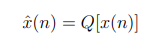
2.2 Quantization and Encoding

Amplitude quantization allow us to represent the discrete-time signal into particular N-bit representation. Obviously, we incurred errors due to 2^N discrete level preference rather an infinite levels in analog signals. The operation is denoted by

The quantizer has L+ 1 decision levels that divides the x(n) range to L intervals. The input must fall within interval I_k. The quantizer assigns a value within this interval, xk to x(n). ∆ represents the quantization resolution or step size and the range of possible values are covered within a step size,

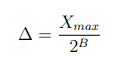
The number of levels L is L = 2^B+1 and the range of the quantizer is R = 2^B+1
· ∆. We define the quantization error,

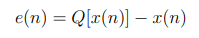
which is bounded by −∆/2 < e(n) < ∆/2. The higher bits minimized the error but cost more to implement.

2.3. Matlab Simulation

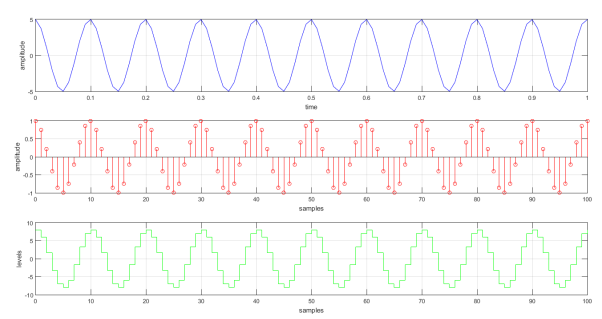
We consider the problem:

A continuous-time signal is given as x(t) = 5cos(20πt + 0.1). Represent the signal in discrete-time.

We start by sampling the signal. The frequency F₀ of the signal is 10 Hz. We set the sampling frequency at 100 Hz, which adheres to the Nyquist rate, Fs ≥ 2F₀. The sampling time Ts is 1/100. We have the sampled signal as

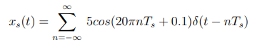
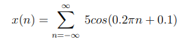
where δ(t − nTs) denotes a unit impulse train that is spaced at Ts. We have x(n) as

Then, we quantized the discrete signal to produce a digital signal. We used a 3-bit quantizer for the task. In MATLAB, we generate the binary code representing the signal. Here is some of the values: 0001000, 0000110, 0000010, 0000011, 0000111, 0001000, 0000110 and 0000010. The plot for each signal is shown in figure.

For the MATLAB script, the equations in the code is modified to the actual equations stated in each problem, which includes the sampling parameters. The script is listed below.

%Continuous=time signal and sampling parameters
f s = 100;
t = 0:1/ f s : 1 ;
xt = 5cos(20*pi*t);

%Discrete-time signal
n = 0 : 1 : 1 0 0 ;
xn =5cos( 0.2*pi*n);

%Quantization and Encoding
qn = max( xn ) / 8;
y=round ( xn/qn ) ;
sgn = uint8( ( si g n ( y ) ’+1) /2 ) ;
xhn =[sgn dec2bin ( abs( y ) , 7 ) ] ; %encode the signal to binary

%plotting signal representation
ax1 = s u b plo t ( 3 , 1 , 1 ) ;
pl o t (t , xt , ’b ’ ) ; g ri d on ;
ax2 = s u b plo t ( 3 , 1 , 2 ) ;
stem (n , xn , ’ r ’ , ’ MarkerSize ’ , 4 ) ; grid on ;
ax3 = s u b plo t ( 3 , 1 , 3 ) ;
stairs(n , xn *(1/ qn ) , ’ g ’ ) ; grid on ;
x l a b e l ( ax1 , ’ time ’ ) ;
x l a b e l ( ax2 , ’ samples ’ ) ;
xlabel( ax3 , ’ samples ’ ) ;
ylabel( ax1 , ’ amplitude ’ ) ;
ylabel( ax2 , ’ amplitude ’ ) ;
ylabel( ax3 , ’ levels ’ ) ;

3. Conclusion

Analog-to-Digital Conversion involves three steps: sampling, quantization and encoding. A convenient way to sample a signal is to multiply it with a periodic impulses or an impulse train. When we sampled signal, we should adhere to the Nyquist rate so that we prevent aliasing. Aliasing happen when the discrete-time signal produce ”aliases” of the continuous signal. Nyquist rate establishes the minimum sampling frequency, which is fs ≥ 2fm. After the continuous signal is sampled, the discrete-time signal is digitized by quantization and encoding. Quantization enables us to represent the the discrete values into N-bit representation. Hence we convert values to 2N discrete level, the representation has innate errors. The errors is minimized when we increased the number of bits.

4. References

1. Gérard Blanchet, Maurice Charbit, Digital Signal and Image Processing Using MATLAB, online access

2. Neal S. Widmer, Gregory L. Moss, Ronald J. Tocci, Digital Systems: Principles and Applications, 12th Edition, online access

3. John W. Leis, Digital Signal Processing Using MATLAB for Students and Researchers. online access