Working with Sparse Data

Shoutout to Python and R Tips

In this article you will find:

• Introduction
• What is sparse data?
• How is data handled with sparse?
• Some methods for sparse matrices
• A small example

Greetings to all!

So far, we've left the Scipy question open as we begin this new arc. This is where we saw some of the operations that we could perform using this library, such as the search for minimums and roots in a function.

However, Scipy is not relegated to this alone, as now we will see a technique widely used in the world of Data Science and Machine Learning, which is the management of dispersed data.

If you want to know how to handle sparse data, just keep reading.

Let's get started!

What is sparse data?

Shoutout to Amir Masoud Sefidian

When we finish with arrays, we are used to seeing a large number of values organized in rows and/or columns in the following way:

[1,2,3]
[4,5,6]
[7,8,9]

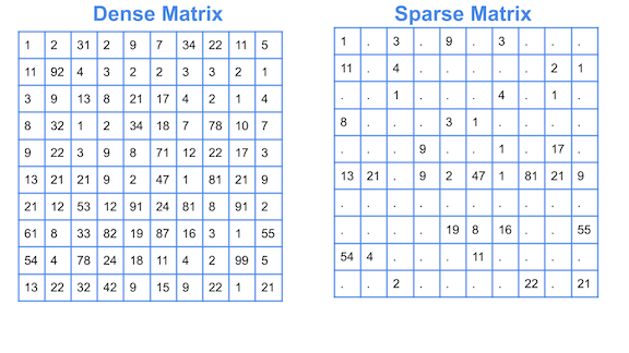
However, there will be certain arrangements where the number of null values (0) greatly exceeds the number of defined values:

[0,0,0,0,0,4,0,0,0,0,3,0,0,0,0,2,1]

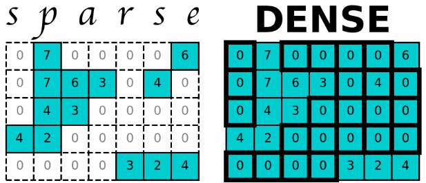
It is these types of arrangements where 0s largely exceed values greater than this, which we call Data Sparse or dispersed data.

Note: Otherwise, if we have an array where the number of non-zero values exceeds those that are zero, it is considered a dense matrix.

Now, if we tried to manage this dispersed data with a library that is not as complex as numpy or Vanilla Python functions, we will realize something:

import numpy as np

arrvar = np.array([0,0,0,0,0,4,0,0,0,0,3,0,0,0,0,2,1])

print(arrvar)

>>>
array([0,0,0,0,0,4,0,0,0,0,3,0,0,0,0,2,1])

If we see this, we will have a couple of problems:

• Working with so many zeros in a conventional array consumes more memory, having to store the 0s as relevant values like 4,2 and 1.
• Makes the job of searching for those addresses where non-null values are more difficult.

We remember that in order to work well with data in Data Science, we must have the information well organized, otherwise we would encounter errors when managing DataSets.

In order to solve all this, we make use of Scipy, specifically its sparse module to manage this dispersed data information.

In this way, we can carry out different operations. From counting the number of non-null values to creating new arrays without zeros, we will be able to perform a large number of tasks with sparse.

Now that we know which library to use, it's time to see it in action.

How is data handled with sparse?

Shoutout to GeeksforGeeks

The main way we will work with sparse data using sparse is by converting the provided arrays into arrays. These matrices can be controlled to our liking with the Sparse methods.

Now, when transforming into a matrix, there are two types of sparse matrices that we can use:

• The csr matrices (Compressed sparse row), which give us better options to remove and work with rows individually.
• The csc (Compressed Sparse Column) matrices, which allow us to work quickly and efficiently with columns.

In order to apply this type of arrays to our program, we must first call numpy to create the initial array:

import numpy as np


arr = np.array([0,0,0,0,2,0,0,4,0,5])

Then, according to the module and type of matrix that we are going to use, we invoke csr_matrix or csc_matrix, which will be the functions required to create one of these matrices.

from scipy import csr_matrix

Now, both csr_matrix and csc_matrix will have a series of parameters, which are:

• The value of the array
• The shape of the matrix (Columns x Rows)
• The type of data the array contains.

csr_matrix(value, shape, datatype)

However, if we provide it with the value of the array it can detect its shape automatically, which will mean that we do not have to enter shape or the datatype most of the time.

Now, if we apply csr_matrix to our example:

import numpy as np
from scipy import csr_matrix


arr = np.array([0,0,0,0,2,0,0,4,0,5])
print(csr_matrix(arr))

>>>
   (0, 4) 2
   (0, 7) 4
   (0, 9) 5

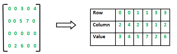
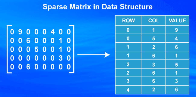
Here we can see that the numbers inside the parentheses will represent the position of the non-null value. For example, for the value of 2, we notice that it is in row 0 (Since it is a single row array) and in column 4.

In case of using the csc_matrix, it would be exactly the same case, where because in this example we are not performing direct operations with rows or columns, we would obtain the same result regardless of the type of matrix.

Some methods for sparse matrices

Shoutout to Javatpoint

In order to be able to move between the large number of zeros that sparse matrices have, both the csr and csc matrices have methods that allow us to access the data we want, among these we have:

Data

When we want to see non-zero data in our sparse matrix, then Data will be the best option, which will take the non-zero values and organize them in the form of a matrix:

import numpy as np
from scipy import csr_matrix


arr = np.array([0,0,0,0,2,0,0,4,0,5])
print(csr_matrix(arr).data)

>>>
[2 4 5]

And if we do it with a two-dimensional array (A matrix)

import numpy as np
from scipy.sparse import csr_matrix

arr = np.array([[0,0,0],[0,2,0],[0,4,5]])

print(csr_matrix(arr).data)

>>>
[2,4,5]

count_nonzero()

As the name implies, with count_nonzero we can count the number of values in our sparse data that do not have the value 0. If we go back to the previous example:

import numpy as np
from scipy.sparse import csr_matrix

arr = np.array([[0,0,0],[0,2,0],[0,4,5]])

print(csr_matrix(arr).count_nonzero())

>>>
3

We can see that we got the number 3, just the number of non-zero values in our array.

eliminate_zeros

How eliminate_zeros works is one of the topics that causes the most confusion among those who start using scipy. We know that data stores all those values that are not 0, that is, it takes the values and stores them somewhere in memory as an 'explicit' value.

Now, what eliminate_zeros does is take explicit values that could have a value of 0 in the data array and eliminate them. If, for example, we changed the value in position 1 of the array in the previous example to 0:

import numpy as np
from scipy.sparse import csr_matrix

arr = np.array([[0,0,0],[0,2,0],[0,4,5]])
arr_mat = csr_matrix(arr)
arr_mat.data[1] = 0

print(arr_mat.data)

>>>
[2,0,5]

Now, if we use eliminate_zeros, the 0 in data will be deleted and only 2 and 5 will be left.

import numpy as np
from scipy.sparse import csr_matrix

arr = np.array([[0,0,0],[0,2,0],[0,4,5]])
arr_mat = csr_matrix(arr)
arr_mat.data[1] = 0
arr_mat.eliminate_zeros()

print(arr_mat.data)

>>>
[2 5]

This deletes this explicit value stored in memory. If we check the value of arr_mat now:

print(arr_mat)

(1, 1) 2
(2, 2) 5

And we have the deleted value.

tocsc()

If we have an array of type csr and we want to change to csc to perform a specific operation, we have a specific method to do this: tocsc()

To create the new array, we just have to insert a new variable and apply the method to our csr list:

1starray = np.array([0,0,1],[0,0,2],[0,0,0])

csr_array = csr_matrix(1starray)
csc_array = csr_array.tocsc()

In this way, if we write the code and execute, we can see the difference when writing the type:

import numpy as np
from scipy.sparse import csr_matrix

firstarray = np.array([[0,0,1],[0,0,2],[0,0,0]])

csr_array = csr_matrix(firstarray)
csc_array = csr_array.tocsc()

print(type(csr_array))
print(type(csc_array))

>>>
<class 'scipy.sparse.csr.csr_matrix'>
<class 'scipy.sparse.csc.csc_matrix'>

A small example

To conclude this lesson, we will see a small example of the potential that Scipy can promise us when working with dispersed data. Let's say we are given an array of numbers, with random numbers from 1 to 9. In this case, we want all values of 1, so we can have two options:

• Create an additional array and every time the value of a cell is 1, add it to this array.
• Make all values other than 1 0 and then use csr_matrix to get all values 1.

Precisely, we will do the second. For this, the first thing we will have to do is import numpy and the csr_matrix function. Then, we determine the value of the matrix, which in this case will be the following:

import numpy as np
from scipy.sparse import csr_matrix

matrix = [[3,3,1],[5,6,1],[7,8,1]]

Then, through a for loop nested within another for loop, we will search the rows, and within the rows, we will search for the cells that have the value of 1. For this, we apply a conditional, where if the condition is met, It will notify us, and if it is not met, it replaces the values in the index with 0.

import numpy as np
from scipy.sparse import csr_matrix

matrix = [[3,3,1],[5,6,1],[7,8,1]]

for row in matrix:
     for column in row:
         if column == 1:
             print('Here\'s a 1')
         else:
             matrix[matrix.index(row)][row.index(column)] = 0

If we see how the matrix would look, we will have:

[[0, 0, 1], [0, 0, 1], [0, 0, 1]]

With which, we almost have the arrangement we want. Now, what remains is to convert this list into a numpy array so that we can apply the csr_matrix to it.

npmatrix = np.array(matrix)

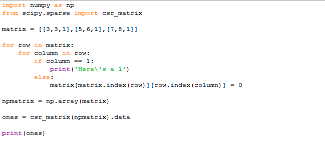
And then, with the data method, we get the values we want:

import numpy as np
from scipy.sparse import csr_matrix

matrix = [[3,3,1],[5,6,1],[7,8,1]]

for row in matrix:
     for column in row:
         if column == 1:
             print('Here\'s a 1')
         else:
             matrix[matrix.index(row)][row.index(column)] = 0

npmatrix = np.array(matrix)

ones = csr_matrix(npmatrix).data

print(ones)

>>>
Here's a 1
Here's a 1
Here's a 1

[1 1 1]

With which we have the values we want.

The management of dispersed data will be an important tool that will allow us to categorize data that we must use when we learn machine learning or some other algorithm.

In this way, I hope that the information provided has been helpful, letting you know that there is more than one way to work with arrangements where the conditions are not favorable.

I invite you to make your own examples and test the potential of sparse.

See you!

Thank you for your support and good luck!

Trabajando con Datos Dispersos

Shoutout to Python and R Tips

En este artículo encontrarás:

• Introducción
• ¿Qué son los datos dispersos?
• ¿Cómo se manejan los datos con sparse?
• Algunos métodos para matrices dispersas
• Un pequeño ejemplo

¡Un saludo a todos!

Hasta ahora, hemos dejado la interrogante de Scipy abierta al iniciar este nuevo arco. Aquí es donde vimos algunas de las operaciones que podíamos realizar empleando esta librería, como lo son la busqueda de mínimos y raíces en una función.

Sin embargo, scipy no se relega solo a esto, pues ahora veremos una técnica muy empleada en el mundo del Data Science y el Machine Learning que es el manejo de datos dispersos.

Si quieres saber como manejar datos dispersos, solo tienes que seguir leyendo.

¡Comencemos!

¿Qué son los datos dispersos?

Shoutout to Amir Masoud Sefidian

Cuando terminamos con arreglos, estamos acostumbrados a ver una gran cantidad de valores organizados en filas y/o columnas de la siguiente forma:

[1,2,3]
[4,5,6]
[7,8,9]

Sin embargo, habrán ciertos arreglos donde el número de valores nulos (0) supere de gran manera a la cantidad de valores definidos:

[0,0,0,0,0,4,0,0,0,0,3,0,0,0,0,2,1]

Es a estos tipos de arreglos donde los 0 superan en gran mayoría a los valores mayores a este que llamamos Data Sparse o de datos dispersos.

Nota: De otra forma, si tenemos un arreglo donde el número de valores que no sean cero superan a aquellos que sean cero, se considera una matriz densa.

Ahora bien, si trataramos de manejar estos datos dispersos con una librería no tan compleja como puede ser numpy o las funciones del Python Vanilla, nos daremos cuenta de algo:

import numpy as np

arrvar = np.array([0,0,0,0,0,4,0,0,0,0,3,0,0,0,0,2,1])

print(arrvar)

>>>
array([0,0,0,0,0,4,0,0,0,0,3,0,0,0,0,2,1])

Si vemos esto, tendremos un par de inconvenientes:

• El trabajar con tantos ceros en un arreglo convencional consume más memoria, al tener que almacenar los 0 como valores relevantes al igual que 4,2 y 1.
• Hace más difícil el trabajo de buscar aquellas direcciones donde están los valores no nulos.

Recordamos que en orden de trabajar bien con datos en Data Science, debemos de tener la información bien ordenada, de otra forma nos encontraríamos con errores al manejar los DataSets.

En orden de solventar todo esto, hacemos uso de scipy, específicamente su módulo sparse para manejar información estos datos dispersos.

De esta forma, podremos realizar distintas operaciones. Desde contar la cantidad de valores no nulos hasta crear nuevas matrices sin ceros, podremos realizar una gran cantidad de tareas con sparse.

Ahora que sabemos que librería usar, es tiempo de verla en acción.

¿Cómo se manejan los datos con sparse?

Shoutout to GeeksforGeeks

La principal manera en la que trabajaremos con los datos dispersos usando sparse es al convertir los arreglos proporcionados en matrices. Estas matrices podrán ser controladas a nuestro gusto con los métodos de Sparse.

Ahora bien, al transformar en matriz, existen dos tipos de matrices dispersas que podemos usar:

• Las matrices csr (Compressed sparse row), las cuales nos brindan mejores opciones para retirar y trabajar con filas de manera individual.
• Las matrices csc (Compressed Sparse Column), que nos permite trabajar de manera rápida y eficiente con columnas.

En orden de aplicar este tipo de matrices a nuestro programa, primero debemos de llamar a numpy para la creación del arreglo inicial:

import numpy as np


arr = np.array([0,0,0,0,2,0,0,4,0,5])

Luego, de acuerdo al módulo y tipo de matriz que vamos a usar, invocamos a csr_matrix o csc_matrix, que serán las funciones requeridos para crear una de estas matrices.

from scipy import csr_matrix

Ahora bien, tanto csr_matrix como csc_matrix tendrán una serie de parámetros, los cuales son:

• El valor de la matriz
• La forma de la matriz (Columnas x Filas)
• El tipo de datos que contiene la matriz.

csr_matrix(value, shape, datatype)

Sin embargo, si le proporcionamos el valor de la matriz este puede detectar su forma automáticamente, lo que hará que no tengamos que colocar shape ni el datatype la mayoría de las veces.

Ahora bien, si aplicamos csr_matrix a nuestro ejemplo:

import numpy as np
from scipy import csr_matrix


arr = np.array([0,0,0,0,2,0,0,4,0,5])
print(csr_matrix(arr))

>>>
  (0, 4)    2
  (0, 7)    4
  (0, 9)    5

Aquí podemos ver que los números dentro del paréntesis nos representarán la posición del valor no nulo. Por ejemplo, para el valor de 2, notamos que está en la fila 0 (Ya que es un arreglo de una sola fila) y en la columna 4.

En caso de usar las csc_matrix, sería exactamente el mismo caso, donde debido a que en este ejemplo no estamos realizando operaciones directas con filas o columnas, obtendríamos el mismo resultado independientemente del tipo de matriz.

Algunos métodos para matrices dispersas

Shoutout to Javatpoint

En orden de poder movernos entre la gran cantidad de ceros que poseen las matrices dispersas, tanto las matrices csr como csc poseen métodos que nos permiten acceder a los datos que deseamos, entre estos tenemos:

Data

Cuando queremos ver los datos que no tengan cero en nuestra matriz dispersa, entonces Data será la mejor opción, la cual tomará los valores no nulos y los organizará en forma de matriz:

import numpy as np
from scipy import csr_matrix


arr = np.array([0,0,0,0,2,0,0,4,0,5])
print(csr_matrix(arr).data)

>>>
[2 4 5]

Y si lo hacemos con un arreglo de dos dimensiones (Una matriz)

import numpy as np
from scipy.sparse import csr_matrix

arr = np.array([[0,0,0],[0,2,0],[0,4,5]])

print(csr_matrix(arr).data)

>>>
[2,4,5]

count_nonzero()

Como su nombre lo indica, con count_nonzero podemos contar la cantidad de valores en nuestros datos dispersos que no tienen el valor de 0. Si volvemos al ejemplo anterior:

import numpy as np
from scipy.sparse import csr_matrix

arr = np.array([[0,0,0],[0,2,0],[0,4,5]])

print(csr_matrix(arr).count_nonzero())

>>>
3

Podemos ver que obtuvimos el número 3, justo la cantidad de valores que no son cero en nuestra matriz.

eliminate_zeros

El funcionamiento de eliminate_zeros es uno de los tópicos que causa más confusión entre aquellos que comienzan a usar scipy. Sabemos que data guarda todos aquellos valores que no son 0, es decir, toma los valores y los almacena en algún lugar de memoria como un valor 'explícito'.

Ahora bien, lo que hace eliminate_zeros es tomar valores explícitos que puedan tener un valor de 0 en el arreglo de data y eliminarlos. Si por ejemplo, cambiaramos el valor en la posición 1 del arreglo del ejemplo anterior por 0:

import numpy as np
from scipy.sparse import csr_matrix

arr = np.array([[0,0,0],[0,2,0],[0,4,5]])
arr_mat = csr_matrix(arr)
arr_mat.data[1] = 0

print(arr_mat.data)

>>>
[2,0,5]

Ahora, si usamos eliminate_zeros, el 0 en data se borrará y solo quedará 2 y 5.

import numpy as np
from scipy.sparse import csr_matrix

arr = np.array([[0,0,0],[0,2,0],[0,4,5]])
arr_mat = csr_matrix(arr)
arr_mat.data[1] = 0
arr_mat.eliminate_zeros()

print(arr_mat.data)

>>>
[2 5]

Con lo que se borra este valor explícito guardado en la memoria. Si revisamos el valor de arr_mat ahora:

print(arr_mat)

(1, 1)  2
(2, 2)  5

Y tenemos el valor borrado.

tocsc()

Si tenemos una matriz de tipo csr y queremos hacer el cambio a csc para realizar una operación específica, tenemos un método específico para realizar esto: tocsc()

Para crear la nueva matriz, solo tenemos que insertar una nueva variable y aplicar el método a nuestra lista csr:

1starray = np.array([0,0,1],[0,0,2],[0,0,0])

csr_array = csr_matrix(1starray)
csc_array = csr_array.tocsc()

De esta forma, si escribimos el código y ejecutamos, podremos ver la diferencia al escribir el tipo:

import numpy as np
from scipy.sparse import csr_matrix

firstarray = np.array([[0,0,1],[0,0,2],[0,0,0]])

csr_array = csr_matrix(firstarray)
csc_array = csr_array.tocsc()

print(type(csr_array))
print(type(csc_array))

>>>
<class 'scipy.sparse.csr.csr_matrix'>
<class 'scipy.sparse.csc.csc_matrix'>

Un pequeño ejemplo

Para concluir esta lesión, veremos un pequeño ejemplo del potencial que nos puede prometer scipy al trabajar con datos dispersos. Digamos que nos proporcionan una matriz de números, con números del 1 al 9 al azar. En este caso, queremos todos los valores de 1, por lo que podemos tener dos opciones:

• Crear un arreglo adicional y cada vez que el valor de una celda sea 1, añadirlo a este arreglo.
• Hacer 0 todos los valores que no sean 1 y luego usar csr_matrix para obtener todos los valores de 1.

Precisamente, haremos lo segundo. Para esto, lo primero que tendremos que hacer es importar numpy y la función csr_matrix. Luego, determinamos el valor de la matriz, que en este caso serán los siguientes:

import numpy as np
from scipy.sparse import csr_matrix

matrix = [[3,3,1],[5,6,1],[7,8,1]]

Luego, por medio de un ciclo for anidado dentro de otro ciclo for, buscaremos en las filas, y dentro de las filas, buscaremos las celdas que tengan el valor de 1. Para esto, aplicamos un condicional, donde si se cumple la condición, nos avisará, y en caso de no cumplirse, reemplaza los valores en el índice por 0.

import numpy as np
from scipy.sparse import csr_matrix

matrix = [[3,3,1],[5,6,1],[7,8,1]]

for row in matrix:
    for column in row:
        if column == 1:
            print('Here\'s a 1')
        else:
            matrix[matrix.index(row)][row.index(column)] = 0

Si vemos como quedaría la matriz, tendremos:

[[0, 0, 1], [0, 0, 1], [0, 0, 1]]

Con lo cual, ya casi tenemos el arreglo que queremos. Ahora, lo que resta es convertir esta lista en un arreglo de numpy para poder aplicarle el csr_matrix.

npmatrix = np.array(matrix)

Y luego, con el método data, obtenemos los valores que queremos:

import numpy as np
from scipy.sparse import csr_matrix

matrix = [[3,3,1],[5,6,1],[7,8,1]]

for row in matrix:
    for column in row:
        if column == 1:
            print('Here\'s a 1')
        else:
            matrix[matrix.index(row)][row.index(column)] = 0

npmatrix = np.array(matrix)

ones = csr_matrix(npmatrix).data

print(ones)

>>>
Here's a 1
Here's a 1
Here's a 1

[1 1 1]

Con lo que tenemos los valores que queremos.

El manejo de datos dispersos será una herramienta importante que nos permitirá categorizar datos que debamos usar cuando aprendamos machine learning o algún otro algoritmo.

De esta forma, espero que la información prevista haya sido de ayuda, haciéndote saber que hay más de una forma de trabajar con arreglos donde las condiciones no favorables.

Te invito a hacer tus propios ejemplos y probar el potencial de sparse.

¡Nos vemos!

¡Gracias por tu apoyo y buena suerte!