Looking for the Shortest Path

Shoutout to O'Reilly

In this article you'll find:

• Introduction
• What are adjacent matrices?
• connected_components()
• Dijkstra algorithm

Greetings to all!

In this edition of Coding Basics we continue our stay in Scipy, seeing the complex operations that we can perform with it, such as managing scattered data and obtaining data whose value is not 0.

However, the power of this library does not end here. That is why today we will work with adjacent matrices and we will see some of the operations we can perform with them.

This way, if you want to work with all types of data in Scipy, just keep reading.

Let's get started!

What is an adjacent matrix?

Shoutout to ResearchGate

Before starting to work with the Dijkstra and connected_components functions, we must know what an adjacent matrix is.

An adjacent matrix is a matrix that has the same number of columns and rows (nxn), where this number refers to the number of elements in a graph. This means that if we have 6 elements in our graph, then we will have an adjacent 6x6 matrix.

However, this does not fully explain what this matrix does. In order to understand what it is used for, we must take into account the concept of adjacent:

That is very close or attached to something else

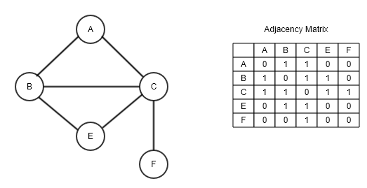
In this case, if two elements are adjacent, this means that they are joined. For example, if we look at the following graph, which is closely related to Fibonacci mounds, we can see that these circles (Better known as nodes), which will be our elements, are connected to other circles. This means that they are adjacent.

Shoutout to Discovering Python & R

For example, if we take node A, we will see that it is adjacent to both B and C and E.

It is precisely these adjacencies and connections with which we create our matrix, where, following the previous graph, observing the connections between the elements, we would have the matrix:

   A|B|C|D|E
A[0,1,1,0,1]
B[1,0,1,0,0]
C[1,1,0,1,1]
D[0,0,1,0,0]
E[1,0,1,0,0]

Here, we can see that each column and each row represents an element quite similar to searching for correlations in Pandas.

Analyzing this matrix, we can see that the 1's in the columns of a particular row will show us if they are connected.

Note: Since A and A are the same element, a 0 is placed in this cell. This is repeated for the rest of the rows in the column of the same index.

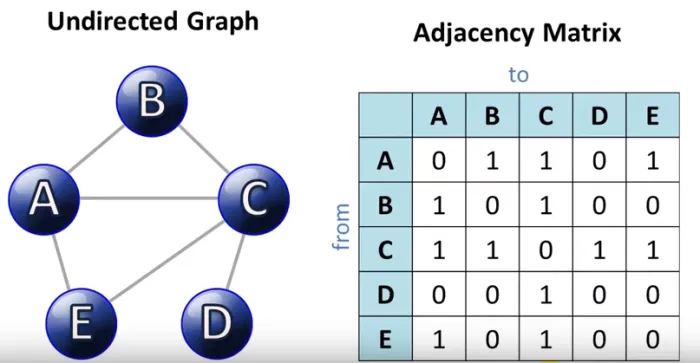
However, adjacent matrices are not only limited to these types of graphs. You see, in this case, because the lines connecting the nodes (called edges) do not have arrows, we can say that this is an undirected matrix, where the elements are interconnected and if, for example, we found that column B is connected to row A and has a 1, then column A in row B will also have a 1.

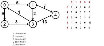
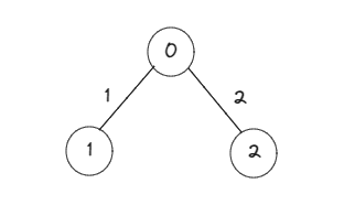
We also have those matrices where the direction of the matrix is specified, which we call directed adjacent matrices. In the following graph, we can see that the elements have arrows in the direction from one node to another. If we saw the resulting matrix:

Shoutout to Fahadul Shadhin in Medium

Here we can see that node 0 connects in only one direction to 1 and 2, which is why the arrow is here, as do 1 to 4, 2 to 3, and 3 to 4. This would translate into matrix form as We can see it in the image, where row 0 has connections (1) in column 1 and 2. However, neither row 1 nor row 2 have connections in cell 0.

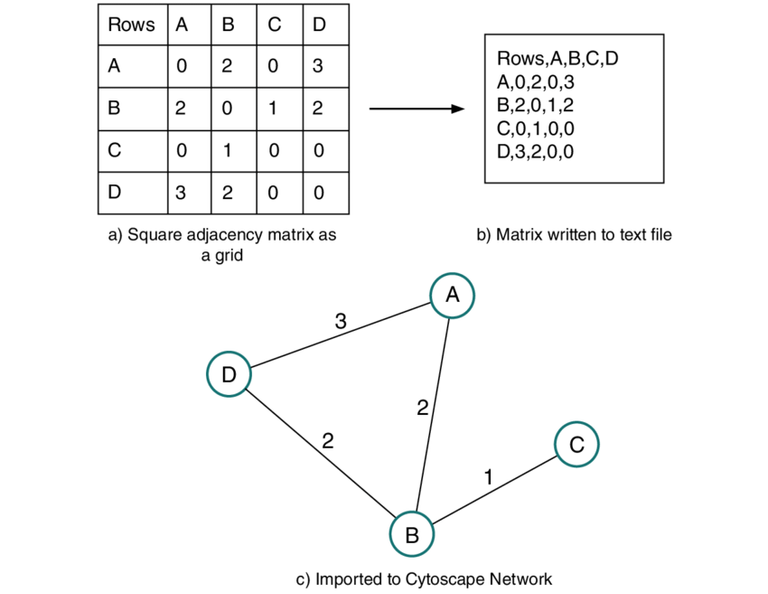
In addition to this, we will have cases where we will see numbers on the edges that connect the nodes, which will affect the way the matrix is represented, where instead of placing the values of 1, we will place these numbers. This is what is known as an adjacent matrix of a weighted graph:

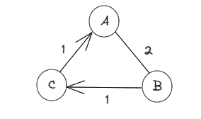
   ABC
A[0,2,0]
B[2,0,1]
C[1,0,0]

These are the values between the nodes that we call "cost".

Note: Arrays that only have costs of 1 are adjacent arrays of unweighted graphs.

Now that we know this, we can move on to study what the Dijkstra and connected_components functions are.

connected_components()

Shoutout to snoob dogg

Based on the connected_components statement, this is a fairly simple operation. What we do with this function is find all the elements that are connected by using connected_components() which takes the name of the array as a parameter. However, if we were to use this function with an adjacent 3 by 3 matrix, we would see the following:

import numpy as np
from scipy.sparse.csgraph import connected_components
from scipy.sparse import csr_matrix

arr = np.array([
   [0, 1, 2],
   [1, 0, 0],
   [200]
])

newarr = csr_matrix(arr)

print(connected_components(newarr))

We will obtain the following:

(1, array([0, 0, 0], dtype=int32))

"What is this data? I thought I was going to get information about the connected items."

This is the information about the connected data. The first is the number of elements that are connected to each other forming a vertex, assigning the index of 0, which is why we also have an array with three 0's (Our three elements) and the DataType of int32 since they are integers.

However, if we increase the number of vertices to 3, creating 6 more elements, of which the first three will be connected to each other but isolated from 0, 1 and 2 as well as from the last ones (6,7 and 8), while The last three are connected to each other but are isolated from 0,1 and 2 as well as from 3,4 and 5, we will have:

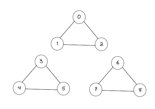
We can see that the adjacent matrix representation would be the following:

[
   [0, 1, 1, 0,0,0, 0,0,0],
   [1, 0, 1, 0,0,0, 0,0,0],
   [1, 1, 0, 0,0,0, 0,0,0],
   [0, 0, 0, 0,1,1, 0,0,0],
   [0, 0, 0, 1,0,1, 0,0,0],
   [0, 0, 0, 1,1,0, 0,0,0],
   [0, 0, 0, 0,0,0, 0,1,1],
   [0, 0, 0, 0,0,0, 1,0,0],
   [0, 0, 0, 0,0,0, 1,0,0],
]

And that when running the code for connected_components:

import numpy as np
from scipy.sparse.csgraph import connected_components
from scipy.sparse import csr_matrix

arr = np.array([
   [0, 1, 1, 0,0,0, 0,0,0],
   [1, 0, 1, 0,0,0, 0,0,0],
   [1, 1, 0, 0,0,0, 0,0,0],
   [0, 0, 0, 0,1,1, 0,0,0],
   [0, 0, 0, 1,0,1, 0,0,0],
   [0, 0, 0, 1,1,0, 0,0,0],
   [0, 0, 0, 0,0,0, 0,1,1],
   [0, 0, 0, 0,0,0, 1,0,0],
   [0, 0, 0, 0,0,0, 1,0,0],
])

newarr = csr_matrix(arr)

print(connected_components(newarr))

(3, array([0, 0, 0, 1, 1, 1, 2, 2, 2], dtype=int32))

Here, we can see that as the number of elements interconnected with each other forming vertices increases, so do the results of our connected_components, where we now identify 3 different vertices.

Dijkstra

Shoutout to avrilomics

Another method that at first glance may seem simple. However, we must take special consideration and analyze first.

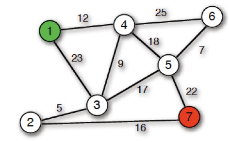
What Dijkstra does is that it allows us to obtain the shortest or lowest cost path from one element to another. In this way, if we analyze the following graph:

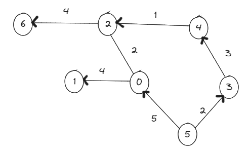
We can see that this is a heavy directed graph. Here, we will see that there are nodes pointing towards other nodes. But, what would happen if we wanted to find the distance or path from one node to another?

For this, we must take into account two things, the direction of the edges and their cost.

For example, if we select a node as our origin, say 5, and we want to find the shortest path to 2, we will have to compare which of the two paths (Going through 3 and then 4 or going through 0) has the lower cost .

If we count the path that passes through 0 before reaching 2, we will see that in the first edge, we will have a cost of 5. Then, when going from 0 to 2, we add to this cost of 5 a value of 2, having a total cost of 7. Not bad. However, let's look at the alternative path.

We see that from 5 to 3, we have a cost of 2 and that when going from 3 to 4, one of 3 is added to this, obtaining 5, and finally when going from 4 to 2, adding 1 and having a total of 6. It is then that we can conclude that the shortest path from 5 to 2 has a cost of 6, which is part of the data we would see when using Dijkstra.

To use the dijkstra function, we must take into account its parameters, which are:

• The name of the array (required).
• directed (optional), this is a boolean value with which we tell Dijkstra if it should search for the shortest path in an adjacent directed array (If True) or undirected (If False).
• indices (optional), which will allow us to know the shortest paths from the node that we specify to the rest of the nodes.
• return_predecessors (Optional), which will also allow us to know which was the last node passed through before reaching the target node.
• unweighted (optional), here we specify to dijkstra that I did not take cost into account, which is why now as the shortest path, it will only take the path with the least number of edges.

Now, if we use a single parameter (The matrix), to get the shortest path from one node to another in the graph shown above:

[0,4,2,0,0,0,0],
[0,0,0,0,0,0,0],
[2,0,0,0,0,0,4],
[0,0,0,0,3,0,0],
[0,0,1,0,0,0,0],
[5,0,0,2,0,0,0],
[0,0,4,0,0,0,0]

That when written in a program it would return the following:

import numpy as np
from scipy.sparse.csgraph import dijkstra
from scipy.sparse import csr_matrix

adj_arr = np.array([
   [0,4,2,0,0,0,0],
   [0,0,0,0,0,0,0],
   [2,0,0,0,0,0,4],
   [0,0,0,0,3,0,0],
   [0,0,1,0,0,0,0],
   [5,0,0,2,0,0,0],
   [0,0,4,0,0,0,0]
])

matr_arr = csr_matrix(adj_arr)

print(dijkstra(matr_arr))

>>>
[[ 0. 4. 2. inf inf inf 6.]
  [inf 0. inf inf inf inf inf]
  [ 2. 6. 0. inf inf inf 4.]
  [ 6. 10. 4. 0. 3. inf 8.]
  [ 3. 7. 1. inf 0. inf 5.]
  [5.9.6.2.5.0.10.]
  [ 6. 10. 4. inf inf inf 0.]]

This resulting matrix simply shows us the total cost of the shortest path to a particular node. If we make this easier by placing the columns and rows of each node:

    0 1 2 3 4 5 6
0[ 0. 4. 2. inf inf inf 6.]
1[inf 0. inf inf inf inf inf]
2[ 2. 6. 0. inf inf inf 4.]
3[ 6. 10. 4. 0. 3. inf 8.]
4[ 3. 7. 1. inf 0. inf 5.]
5[ 5. 9. 6. 2. 5. 0. 10.]
6[ 6. 10. 4. inf inf inf 0.]

Thus, if we take into account the first row (0), we can see that the shortest path to 0 has a cost of 0, since they are the same node. Similarly:

• The shortest path from 0 to 1 has a cost of 4.
• The shortest path from 0 to 2 has a cost of 2.
• The shortest path from 0 to 3 has infinite cost because they are not connected. This is repeated for 4 and 5.
• The shortest path from 0 to 6 has a cost of 6.

All of these can be verified if you look at the graph. Likewise, if we look at the other rows, we see the costs of the shortest paths between elements.

Now, if we use more parameters, we can see more interesting things:

print(dijkstra(matr_arr, return_predecessors=True, indices=0))

>>>
(array([ 0., 4., 2., inf, inf, inf, 6.]), array([-9999, 0, 0, -9999, -9999, -9999, 2], dtype=int32) )

Here, if we look at the first arrangement, we can see that we have the costs of short paths to other nodes, but only from node 0. This is because we set the parameter indices=0, which will return only the connections of the node in the index we place.

In the same way, we obtain an additional array, which will show us the value of the node predecessor to the index we want to find. For example, if we look at the graph, we see that the node preceding node 1 is 0, which is reflected in this matrix in position 1.

Thus, we can find the shortest path in an adjacent graph using Scipy.

Even if there are other methods to find the path with the lowest cost between nodes, such as the Floyd Warshall and Bellman Ford algorithms, with the proposed commands we can handle ourselves with complete confidence when working with adjacent graphs.

Thus, after reading this article, you will have mastered:

• How to determine the number of vertices or elements interconnected with each other.
• The shortest path from one node to another.

Things that will be of great help to you when learning Machine Learning. In this way, I encourage you to put into practice the knowledge acquired in this lesson. Without more to say.

Thank you for your support and good luck!

Buscando el Camino más corto

Shoutout to O'Reilly

In this article you'll find:

• Introducción
• ¿Qué son las matrices adyacentes?
• connected_components()
• Algoritmo Dijkstra

¡Un saludo a todos!

En esta edición de Coding Basics continuamos con nuestra estadía en Scipy, viendo las operaciones complejas que podemos realizar con esta, como el manejo de datos dispersos y la obtención de aquellos datos cuyo valor no es 0.

Sin embargo, el poder de esta librería no termina aquí. Es por eso, que hoy trabajaremos con matrices adyacentes y veremos algunas de las operaciones que podemos realizar con estos.

De esta forma, si deseas trabajar con todo tipo de datos en Scipy, solo tienes que seguir leyendo.

¡Comencemos!

¿Qué es una matriz adyacente?

Shoutout to ResearchGate

Antes de pasar a trabajar con las funciones Dijkstra y connected_components, debemos de saber que es una matriz adyacente.

Una matriz adyacente es una matriz que tiene el mismo número de columnas y filas (nxn), donde este número se refiere a la cantidad de elementos en una gráfica. Esto quiere decir, que si tenemos 6 elementos en nuestra gráfica, entonces tendremos una matriz adyacente de 6x6.

Sin embargo, esto no explica en su totalidad lo que hace esta matriz. En orden de entender para que es usada, debemos de tener en cuenta el concepto de adyacente:

Que está muy próximo o unido a otra cosa

En este caso, si dos elementos son adyacentes, esto quiere decir que están unidos. Por ejemplo, si observamos la siguiente gráfica, la cual guarda un gran parentesco con montículos de Fibonacci, podremos ver que estos círculos (Mejor conocidos como nodos), que serán nuestros elementos, se encuentran conectados a otros círculos. Esto quiere decir que son adyacentes.

Shoutout to Discovering Python & R

Por ejemplo, si tomamos el nodo A, veremos que este es adyacente tanto a B y C como a E.

Es precisamente estas adyacencias y conexiones con las que creamos nuestra matriz, donde, siguiendo la gráfica anterior, observando las conexiones entre los elementos, tendríamos la matriz:

  A|B|C|D|E
A[0,1,1,0,1]
B[1,0,1,0,0]
C[1,1,0,1,1]
D[0,0,1,0,0]
E[1,0,1,0,0]

Aquí, podemos ver que cada columna y cada fila representa un elemento de manera bastante similar a la busqueda de correlaciones en Pandas.

Analizando esta matriz, podemos ver que los 1 en las columnas de una fila particular nos mostrará si se encuentran conectados.

Nota: Ya que A y A son el mismo elemento, se coloca un 0 en esta celda. Esto se repite para el resto de filas en la columna del mismo índice.

Sin embargo, las matrices adyacentes no solo se limitan a este tipos de gráficos. Verás, en este caso, debido a que las líneas que conectan los nodos (Llamados edges) no tienen flechas, se puede decir que esta es una matriz no dirigida, donde los elementos están interconectados y si, por ejemplo, encontraramos que la columna B está conectada a la fila A y tiene un 1, entonces la columna A en la fila B también tendrá un 1.

También tenemos aquellas matrices donde la dirección de la matriz se especifica, a las cuales llamamos matrices adyacentes dirigidas. En la siguiente gráfica, podemos ver que los elementos tienen flechas en el sentido de un nodo hacia otro. Si vieramos la matriz resultante:

Shoutout to Fahadul Shadhin in Medium

Aquí podemos ver que el nodo 0 se conecta en una sola dirección a 1 y 2, razón por la cual la flecha está aquí, al igual que 1 a 4, 2 a 3 y 3 a 4. Esto se traduciría en forma de matriz como lo podemos observar en la imagen, donde la fila 0 presenta conexiones (1) en la columna 1 y 2. Sin embargo, ni la fila 1 ni la fila 2 tienen conexiones en la celda 0.

Además de esto, tendremos casos donde veremos números en los edges que conectan a los nodos, los cuales afectarán la forma en que se representa la matriz, donde en vez de colocar los valores de 1, colocaremos estos números. Esto es lo que se conoce como una matriz adyacente de un gráfico pesado o weighted:

  A B C
A[0,2,0]
B[2,0,1]
C[1,0,0]

Son estos valores que hay entre los nodos a los cuales llamamos "costo".

Nota: Las matrices que solo tienen costos de 1 son matrices adyacentes de gráficos no pesados o unweighted.

Ahora que sabemos esto, podemos pasar a estudiar que son las funciones Dijkstra y connected_components.

connected_components()

Shoutout to snoob dogg

Según el enunciado de connected_components, esta es una operación bastante sencilla. Lo que hacemos con esta función es encontrar todos los elementos que están conectados al usar connected_components() que toma como parámetro el nombre de la matriz. Sin embargo, si usaramos esta función con una matriz adyacente de 3 por 3, veríamos lo siguiente:

import numpy as np
from scipy.sparse.csgraph import connected_components
from scipy.sparse import csr_matrix

arr = np.array([
  [0, 1, 2],
  [1, 0, 0],
  [2, 0, 0]
])

newarr = csr_matrix(arr)

print(connected_components(newarr))

Obtendremos lo siguiente:

(1, array([0, 0, 0], dtype=int32))

"¿Qué son estos datos? Pensaba que iba a obtener información sobre los elementos conectados."

Esta es la información sobre los datos conectados. La primera es la cantidad de elementos que se encuentran conectados entre si formando un vertice, asignándole el índice de 0, razón por la que también tenemos un arreglo con tres 0 (Nuestros tres elementos)y el DataType de int32 ya que son enteros.

Sin embargo, si aumentaramos el número de vertices a 3, creando 6 elementos más, de los cuales los primeros tres estarán conectados entre si pero aislados de 0, 1 y 2 así como de los últimos (6,7 y 8), mientras que los últimos tres se conectan entre si pero están aislados de 0,1 y 2 así como de 3,4 y 5, tendremos:

Podemos ver que la representación en matriz adyacente sería la siguiente:

[
  [0, 1, 1, 0,0,0, 0,0,0],
  [1, 0, 1, 0,0,0, 0,0,0],
  [1, 1, 0, 0,0,0, 0,0,0],
  [0, 0, 0, 0,1,1, 0,0,0],
  [0, 0, 0, 1,0,1, 0,0,0],
  [0, 0, 0, 1,1,0, 0,0,0],
  [0, 0, 0, 0,0,0, 0,1,1],
  [0, 0, 0, 0,0,0, 1,0,0],
  [0, 0, 0, 0,0,0, 1,0,0],
]

Y que al ejecutar el código para connected_components:

import numpy as np
from scipy.sparse.csgraph import connected_components
from scipy.sparse import csr_matrix

arr = np.array([
  [0, 1, 1, 0,0,0, 0,0,0],
  [1, 0, 1, 0,0,0, 0,0,0],
  [1, 1, 0, 0,0,0, 0,0,0],
  [0, 0, 0, 0,1,1, 0,0,0],
  [0, 0, 0, 1,0,1, 0,0,0],
  [0, 0, 0, 1,1,0, 0,0,0],
  [0, 0, 0, 0,0,0, 0,1,1],
  [0, 0, 0, 0,0,0, 1,0,0],
  [0, 0, 0, 0,0,0, 1,0,0],
])

newarr = csr_matrix(arr)

print(connected_components(newarr))

(3, array([0, 0, 0, 1, 1, 1, 2, 2, 2], dtype=int32))

Aquí, podemos ver que ya que la cantidad de elementos interconectados entre si formando vertices aumentan, también los hacen los resultados de nuestro connected_components, donde ahora identificamos 3 vertices distintos.

Dijkstra

Shoutout to avrilomics

Otro método que a simple vista puede parecer sencillo. Sin embargo, debemos de tener especial consideración y analizar primero.

Lo que hace Dijkstra es que nos permite obtener el camino más corto o de menor costo de un elemento hacia otro. De esta forma, si analizamos el siguiente gráfico:

Podemos ver que este es un gráfico direccionado pesado. Aquí, veremos que hay nodos apuntando hacia otros nodos. Pero, ¿Qué pasaría si quisieramos hayar la distancia o el camino de un nodo hacia otro?

Para esto, debemos de tomar en cuenta dos cosas, la dirección de los edges y el costo de estos.

Por ejemplo, si seleccionamos un nodo como nuestro origen, digamos el 5, y queremos encontrar el camino más corto hacia 2, tendremos que comparar cual de los dos caminos (El pasar por 3 y luego 4 o pasar por 0) tiene el coste menor.

Si contamos el camino que pasa por el 0 antes de llegar a 2, veremos que en el primer edge, tendremos un costo de 5. Luego, Al pasar del 0 al 2, añadimos a este coste de 5 un valor de 2, teniendo un coste total de 7. Nada mal. Sin embargo, veamos el camino alternativo.

Vemos que del 5 al 3, tenemos un coste de 2 y que al pasar de 3 a 4, se añade a este uno de 3, obteniendo 5, para finalmente al pasar de 4 a 2, añadirle 1 y tener un total de 6. Es entonces, que podemos concluir que el camino más corto de 5 a 2 tiene un costo de 6, lo cual forma parte de los datos que veríamos al usar Dijkstra.

Para usar la función dijkstra, debemos de tomar en cuenta sus parámetros, los cuales son:

• El nombre de la matriz (obligatorio).
• directed (opcional), este es un valor booleano con el que le indicamos a Dijkstra si debe de buscar el camino más corto en una matriz adyacente dirigida (Si es True) o no dirigida (Si es False).
• indices (opcional), que nos permitirá saber los caminos más cortos desde el nodo que especifiquemos hacia el resto de nodos.
• return_predecessors (Opcional), que también nos permitirá saber cual fue el último nodo por donde se pasó antes de llegar al nodo objetivo.
• unweighted (opcional), aquí especificamos a dijkstra que no tomé en cuenta el costo, razón por la cual ahora como camino más corto, solo tomará el camino con la menor cantidad de edges.

Ahora, si usamos un solo parámetro (La matriz), para obtener el camino más corto de un nodo a otro en el gráfico mostrado anteriormente:

[0,4,2,0,0,0,0],
[0,0,0,0,0,0,0],
[2,0,0,0,0,0,4],
[0,0,0,0,3,0,0],
[0,0,1,0,0,0,0],
[5,0,0,2,0,0,0],
[0,0,4,0,0,0,0]

Que al escribirlo en un programa nos retornaría lo siguiente:

import numpy as np
from scipy.sparse.csgraph import dijkstra
from scipy.sparse import csr_matrix

adj_arr = np.array([
  [0,4,2,0,0,0,0],
  [0,0,0,0,0,0,0],
  [2,0,0,0,0,0,4],
  [0,0,0,0,3,0,0],
  [0,0,1,0,0,0,0],
  [5,0,0,2,0,0,0],
  [0,0,4,0,0,0,0]
])

matr_arr = csr_matrix(adj_arr)

print(dijkstra(matr_arr))

>>>
[[ 0.  4.  2. inf inf inf  6.]
 [inf  0. inf inf inf inf inf]
 [ 2.  6.  0. inf inf inf  4.]
 [ 6. 10.  4.  0.  3. inf  8.]
 [ 3.  7.  1. inf  0. inf  5.]
 [ 5.  9.  6.  2.  5.  0. 10.]
 [ 6. 10.  4. inf inf inf  0.]]

Esta matriz resultante simplemente nos muestra el costo en total del camino más corto hacia un nodo particular. Si facilitamos esto colocando las columnas y filas de cada nodo:

   0   1   2   3   4   5   6   
0[ 0.  4.  2. inf inf inf  6.]
1[inf  0. inf inf inf inf inf]
2[ 2.  6.  0. inf inf inf  4.]
3[ 6. 10.  4.  0.  3. inf  8.]
4[ 3.  7.  1. inf  0. inf  5.]
5[ 5.  9.  6.  2.  5.  0. 10.]
6[ 6. 10.  4. inf inf inf  0.]

Así, si tomamos en cuenta la primera fila (0), podemos ver que el camino más corto hacia 0 tiene un coste de 0, ya que son el mismo nodo. De igual forma:

• El camino más corto desde 0 hacia 1 tiene un costo de 4.
• El camino más corto desde 0 hacia 2 tiene un costo de 2.
• El camino más corto desde 0 hacia 3 tiene un costo infinito debido a que no están conectados. Esto se repite para 4 y 5.
• El camino más corto de 0 a 6 tiene un costo de 6.

Todas estas pueden ser comprobadas si se observa el gráfico. De igual forma, si observamos las otras filas, vemos los costes de los caminos más cortos entre elementos.

Ahora bien, si usamos más parámetros, podemos ver cosas más interesantes:

print(dijkstra(matr_arr, return_predecessors=True, indices=0))

>>>
(array([ 0.,  4.,  2., inf, inf, inf,  6.]), array([-9999,     0,     0, -9999, -9999, -9999,     2], dtype=int32))

Aquí, si observamos el primer arreglo, podremos ver que tenemos tenemos los costes de los caminos cortos hacia otros nodos, pero solo desde el nodo 0. Esto debido a que colocamos el parámetro indices=0, que nos devolverá solo las conexiones del nodo en el índice que coloquemos.

De igual forma, obtenemos un arreglo adicional, que nos mostrará el valor del nodo predecesor al índice que queremos encontrar. Por ejemplo, si vemos el gráfico, vemos que el nodo que precede al nodo 1 es 0, lo cual se plasma en esta matriz en la posición 1.

Así, podemos encontrar el camino más corto en un gráfico adyacente por medio de Scipy.

Aún si existen otros métodos para encontrar el camino con el menor costo entre nodos como pueden ser los algoritmos Floyd Warshall y Bellman Ford, con los comandos propuestos podemos manejarnos con total confianza al trabajar con gráficos adyacentes.

Así, tras haber leído este artículo, habrás dominado:

• Como determinar la cantidad de vertices o elementos interconectados entre si.
• El camino más corto de un nodo hacia otro.

Cosas que te serán de gran ayuda al aprender Machine Learning. De esta forma, te animo a poner en práctica los conocimientos adquiridos en esta lección. Sin más que decir.

¡Gracias por tu apoyo y buena suerte!