Some operations with Pandas

Shoutout to GeeksForGeeks

In this article you will find:

• Introduction
• Correlation between columns
• Average of columns
• Median of columns
• Column mode

Greetings to all. In the previous edition of Coding Basics, we talked about how to keep our DataFrames neat so that any program that handles our information does not have any problems when analyzing it.

Now, before moving on to the graphing section, we must take into account some statistical functions that we can apply to solve problems or see additional data about our columns and rows. This is why in the following article, we will address some of these.

If you want to learn how to handle your DataFrames accurately in Pandas, keep reading.

Let's get started!

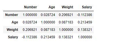
Correlation between columns

Shoutout to Máxima Formación

Shoutout to GeeksForGeeks

Before calculating this, we must know what a correlation is.

A correlation is a statistical measure that allows us to identify how related two variables are.

What it means is that a correlation allows us to determine if two variables (in this case our columns) behave in the same way. For example, if every time a value in column 1 increases a value in column 2 also increases, then we can say that they have the same behavior. Therefore, they have a perfect correlation.

Now, the correlation between values is changing and can range from -1 to 1, -1 being a perfect negative correlation - that is, every time one column increases, the other decreases - and 1, a perfect correlation. If we have a value of 0, this will mean that it is impossible to predict whether one column will increase or decrease each time another column does so.

Shoutout to Máxima Formación

If we want to find the correlation between all the columns of our dataframe, we only have to apply the .corr() method to it, with which it will immediately take the columns of the DataFrame as rows and as columns it will take the other columns with which it is related. For example, if we take the following DataSet, with information about the 5 most popular YouTube Channels:

         Username Subscribers Country Visits Likes
0 tseries 249500000 India 86200 2700
1 MrBeast 183500000 United States 117400000 5300000
2 CoComelon 165500000 United States 7000000 24700
3 SETIndia 162600000 India 15600 166
4 KidsDianaShow 113500000 United States 3900000 12400

Now, we cannot apply a corr, since in order for this method to be applied, the column values must be able to be converted to float (This is why Data Cleaning is important).

To solve this, we just create a new DataFrame, taking the columns with the values we are interested in. In this case, we will take Subscribers, Visits, Likes:

import pandas as pd

df_yt = pd.read_csv('5BiggestYT.csv')

new_yt = df_yt[['Subscribers','Visits','Likes']]

We remember that since it is a two-dimensional array, to take the columns we have to place them inside another array. Now, if we use .corr:

import pandas as pd

df_yt = pd.read_csv('5BiggestYT.csv')

new_yt = df_yt[['Subscribers','Visits','Likes']]

print(new_yt.corr())

>>>
             Subscribers Visits Likes
Subscribers 1.000000 0.070180 0.096131
Visits 0.070180 1.000000 0.998611
Likes 0.096131 0.998611 1.000000

Here, we can see that the rows will represent each column that we have selected and the columns will be their correlation with the others.

In the case of Subscribers, since it is the same column, we will be 100% sure that it will increase if it increases or decrease if it also does so. For visits, we see that the value is very close to 0, so we cannot predict with certainty, which also happens with likes.

The correlation between visits and likes is really close, so we can say that if the number of visits goes down, the number of likes will also go down, which is true.

And here, we can see the correlation between the elements, being able to make predictions based on the data obtained.

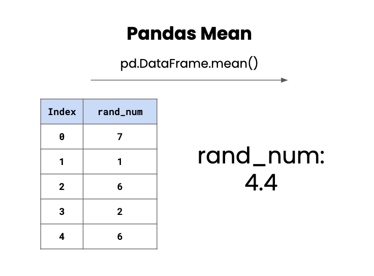
Average of columns

Shoutout to Data Independent

As we saw from the previous article, there are situations where the information for a row may be incomplete or improperly formatted. If we add an additional row to our dataset:

    Subscribers Visits Likes
0 249500000 86200 2700.0
1 183500000 117400000 5300000.0
2 165500000 7000000 24700.0
3 162600000 15600 166.0
4 113500000 3900000 12400.0
5 111000000 100000000 NaN

We know that a possible solution would be to replace the null value with a value that we choose with fillna. However, there will be some cases where we want the information to be consistent or we want to make the best possible prediction regarding the value. For this, we just turn to some statistical functions.

Among these is the mean, which simply refers to an average where all the values in the column are added and divided by the number of indices. To do this operation, we will only have to use the mean() method on the specified column:

import pandas as pd

df_yt = pd.read_csv('5BiggestYT.csv')

mean_likes = df_yt['Likes'].mean()
df_yt.fillna(mean_likes, inplace=True)

print(df_yt)

>>>
         Username Subscribers Country Visits Likes
0 tseries 249500000 India 86200 2700.0
1 MrBeast 183500000 United States 117400000 5300000.0
2 CoComelon 165500000 United States 7000000 24700.0
3 SETIndia 162600000 India 15600 166.0
4 KidsDianaShow 113500000 United States 3900000 12400.0
5 PewDiePie 111000000 Sweden 100000000 1067993.2

Here, we can see that we take the Likes column and apply the mean() to it, finally applying the fillna and thus obtaining the desired value.

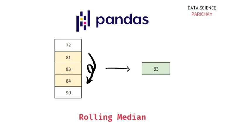
Median of Columns

Shoutout to Data Science Parichay

Another element that we can use to add a value consistent with the data obtained to the null value is the use of the median() method, which calculates the median of the column we select. But what is the median?

The median is the middle number among a group of numbers that are arranged in ascending order. That is, if our data is disordered as we see in our column, the first thing will be to organize it from smallest to smallest:

166, 2700, 12400, 24700, 5300000

In this way, we can quickly decipher that the middle number is 12400. This ease is due to the fact that we are working with an odd number of values. If we were working with an even quantity, we would have to add the two middle numbers and divide by 2 to get the median.

And if we check this by applying the Pandas method for the median: median(), we will have:

import pandas as pd

df_yt = pd.read_csv('5BiggestYT.csv')

median_likes = df_yt['Likes'].median()
df_yt.fillna(median_likes, inplace=True)

print(df_yt)

>>>
  Username Subscribers Country Visits Likes
0 tseries 249500000 India 86200 2700.0
1 MrBeast 183500000 United States 117400000 5300000.0
2 CoComelon 165500000 United States 7000000 24700.0
3 SETIndia 162600000 India 15600 166.0
4 KidsDianaShow 113500000 United States 3900000 12400.0
5 PewDiePie 111000000 Sweden 100000000 12400.0

Column Fashion

Shoutout to GeeksForGeeks

Finally, another statistical operation that we can apply is the mode. What the mode does is that it will take the value that is repeated most frequently. However, in this case each value of the 5 is different, so by default it will take the lowest value:

import pandas as pd

df_yt = pd.read_csv('5BiggestYT.csv')

mode_likes = df_yt['Likes'].mode()[0]
df_yt.fillna(mode_likes, inplace=True)

print(df_yt)

>>>
         Username Subscribers Country Visits Likes
0 tseries 249500000 India 86200 2700.0
1 MrBeast 183500000 United States 117400000 5300000.0
2 CoComelon 165500000 United States 7000000 24700.0
3 SETIndia 162600000 India 15600 166.0
4 KidsDianaShow 113500000 United States 3900000 12400.0
5 PewDiePie 111000000 Sweden 100000000 166.0

However, if we changed the number of Likes of tseries to 12400, the same as KidsDianaShow:

         Username Subscribers Country Visits Likes
0 tseries 249500000 India 86200 12400.0
1 MrBeast 183500000 United States 117400000 5300000.0
2 CoComelon 165500000 United States 7000000 24700.0
3 SETIndia 162600000 India 15600 166.0
4 KidsDianaShow 113500000 United States 3900000 12400.0
5 PewDiePie 111000000 Sweden 100000000 NaN

We will see how fashion is put into practice:

import pandas as pd

df_yt = pd.read_csv('5BiggestYT.csv')

mode_likes = df_yt['Likes'].mode()[0]
df_yt.fillna(mode_likes, inplace=True)

print(df_yt)

>>>
         Username Subscribers Country Visits Likes
0 tseries 249500000 India 86200 12400.0
1 MrBeast 183500000 United States 117400000 5300000.0
2 CoComelon 165500000 United States 7000000 24700.0
3 SETIndia 162600000 India 15600 166.0
4 KidsDianaShow 113500000 United States 3900000 12400.0
5 PewDiePie 111000000 Sweden 100000000 12400.0

As we can see, there is a large number of operations that we can carry out to obtain additional information about the elements within a DataFrame as well as to be able to predict values with them.

This is why Pandas is usually very popular among statistics lovers, being able to make calculations with enormous amounts of information quickly, and after this article, you are already one of them.

However, we are still missing one point: Graphing, which we will see in the next edition of Coding Basics. To see it, stay tuned.

Thank you for your support and good luck!

Algunas operaciones con Pandas

Shoutout to GeeksForGeeks

En este artículo encontrarás:

• Introducción
• Correlación entre columnas
• Media de columnas
• Mediana de columnas
• Moda de columnas

Un saludo a todos. En la edición previa de Coding Basics, hablamos sobre como mantener nuestros DataFrames pulcros para que cualquier programa que maneje nuestra información no tenga inconveniente alguno al analizarla.

Ahora bien, antes de pasar al apartado de graficado, debemos de tomar en cuenta algunas funciones estadísticas que podemos aplicar para resolver problemas o ver datos adicionales sobre nuestras columnas y filas. Es por esto que en el siguiente artículo, abordaremos algunas de estas.

Si quieres aprender como manejar tus DataFrames con precisión en Pandas, sigue leyendo.

¡Comencemos!

Correlación entre columnas

Shoutout to Máxima Formación

Shoutout to GeeksForGeeks

Antes de calcular esto, debemos de saber que es una correlación.

Una correlación es una medida estadística que nos permite identificar que tan relacionadas están dos variables.

Lo que quiere decir es que una correlación nos permite determinar si dos variables (en este caso nuestras columnas) se comportan de la misma forma. Por ejemplo, si cada vez que un valor en la columna 1 aumenta un valor en la columna 2 también lo hace, entonces podemos decir que tienen el mismo comportamiento. Por lo tanto, tienen una correlación perfecta.

Ahora bien, la correlación entre valores es cambiante y puede ir de un rango de -1 a 1, -1 siendo una correlación negativa perfecta --es decir, que cada vez que una columna aumenta, la otra se reduce-- y 1, una correlación perfecta. Si tenemos un valor de 0, esto significara que es imposible predecir si una columna aumentará o se reducirá cada vez que otra lo haga.

Shoutout to Máxima Formación

Si queremos buscar la correlación entre todas las columnas de nuestro dataframe, solo tenemos que aplicar a este el método .corr(), con el que inmediatamente tomará como filas las columnas del DataFrame y como columnas tomará las otras columnas con las que se relaciona. Por ejemplo, si tomamos el siguiente DataSet, con información sobre 5 Canales de Youtube más populares:

        Username  Suscribers        Country     Visits    Likes
0        tseries   249500000          India      86200     2700
1        MrBeast   183500000  United States  117400000  5300000
2      CoComelon   165500000  United States    7000000    24700
3       SETIndia   162600000          India      15600      166
4  KidsDianaShow   113500000  United States    3900000    12400

Ahora, no le podemos aplicar un corr, ya que para que se pueda aplicar este método, los valores de las columna deben de poderse convertir a float (Por esto es que el Data Cleaning es importante).

Para solucionar esto, solo creamos un nuevo DataFrame, tomando las columnas con los valores que nos interesan. En este caso, tomaremos a Subscribers, Visits, Likes:

import pandas as pd

df_yt = pd.read_csv('5BiggestYT.csv')

new_yt = df_yt[['Suscribers','Visits','Likes']]

Recordamos que al ser un arreglo de dos dimensiones, para tomar las columnas tenemos que colocar estas dentro de otro arreglo. Ahora, si usamos .corr:

import pandas as pd

df_yt = pd.read_csv('5BiggestYT.csv')

new_yt = df_yt[['Suscribers','Visits','Likes']]

print(new_yt.corr())

>>>
            Suscribers    Visits     Likes
Suscribers    1.000000  0.070180  0.096131
Visits        0.070180  1.000000  0.998611
Likes         0.096131  0.998611  1.000000

Aquí, podemos ver que las filas representarán cada columna que hemos seleccionado y las columnas, será su correlación con las otras.

En el caso de Suscribers, ya que es la misma columna, tendremos 100% seguro que aumentará si esta aumenta o decrementa si esta también lo hace. Para las visitas, vemos que el valor es muy cercano a 0, por lo que no podemos predecir con seguridad, cosa que también pasa con los likes.

La correlación entre visitas y likeses realmente estrecha, con lo que podemos decir que si baja el número de visitas también bajará el número de likes, algo cierto.

Y aquí, podemos ver la correlación existente entre los elementos, pudiendo hacer predicciones en base a los datos obtenidos.

Media de columnas

Shoutout to Data Independent

Como pudimos observar del artículo anterior, existen situaciones donde la información para una fila puede estar incompleta o tener el formato inadecuado. Si le agregamos una fila adicional a nuestro dataset:

   Suscribers     Visits      Likes
0   249500000      86200     2700.0
1   183500000  117400000  5300000.0
2   165500000    7000000    24700.0
3   162600000      15600      166.0
4   113500000    3900000    12400.0
5   111000000  100000000        NaN

Sabemos que una solución posible sería reemplazar el valor nulo con un valor que escogemos con fillna. Sin embargo, existirán algunos casos donde querremos que la información sea uniforme o queremos hacer la mejor predicción posible con respecto al valor. Para esto, solo recorremos a algunas funciones estadísticas.

Entre estas, se encuentra la media, que simplemente se refiere a un promedio donde se suman todos los valores de la columna y se dividen entre la cantidad de índices. Para hacer esta operación, solo tendremos que usar el método mean() en la columna específicada:

import pandas as pd

df_yt = pd.read_csv('5BiggestYT.csv')

mean_likes = df_yt['Likes'].mean() 
df_yt.fillna(mean_likes, inplace=True)

print(df_yt)

>>>
        Username  Suscribers        Country     Visits      Likes
0        tseries   249500000          India      86200     2700.0
1        MrBeast   183500000  United States  117400000  5300000.0
2      CoComelon   165500000  United States    7000000    24700.0
3       SETIndia   162600000          India      15600      166.0
4  KidsDianaShow   113500000  United States    3900000    12400.0
5      PewDiePie   111000000         Sweden  100000000  1067993.2

Aquí, podemos ver que tomamos la columna Likes y le aplicamos el mean(), finalmente aplicando el fillna y obteniendo así que llenamos el valor deseado.

Mediana de Columnas

Shoutout to Data Science Parichay

Otro elemento que podemos usar para añadir un valor consistente con los datos obtenidos al valor nulo es el uso del método median(), que calcula la mediana de la columna que seleccionemos. Pero, ¿Qué es la mediana?

La mediana es el número del medio entre un grupo de números que se ordenan de forma ascendente. Es decir, que si nuestros datos están desordenados como lo vemos en nuestra columna, lo primera será organizarlos de menor a menor:

166, 2700, 12400, 24700, 5300000

De esta forma, podemos descifrar rápidamente que el número del medio es 12400. Esta facilidad se debe a que trabajamos con una cantidad impar de valores. Si trabajaramos con una cantidad par, tendríamos que sumar los dos números del medio y dividir entre 2 para obtener la mediana.

Y si comprobamos esto aplicando el método de pandas para la mediana: median(), tendremos:

import pandas as pd

df_yt = pd.read_csv('5BiggestYT.csv')

median_likes = df_yt['Likes'].median() 
df_yt.fillna(median_likes, inplace=True)

print(df_yt)

>>>
        Username  Suscribers        Country     Visits      Likes
0        tseries   249500000          India      86200     2700.0
1        MrBeast   183500000  United States  117400000  5300000.0
2      CoComelon   165500000  United States    7000000    24700.0
3       SETIndia   162600000          India      15600      166.0
4  KidsDianaShow   113500000  United States    3900000    12400.0
5      PewDiePie   111000000         Sweden  100000000    12400.0

Moda de Columnas

Shoutout to GeeksForGeeks

Por último, otra de las operaciones estadísticas que podemos aplicar es la de la moda. Lo que hace la moda es que tomará el valor que se repite con mayor frecuencia. Sin embargo, en este caso cada valor de los 5 es distinto, por lo que por defecto tomará el menor valor:

import pandas as pd

df_yt = pd.read_csv('5BiggestYT.csv')

mode_likes = df_yt['Likes'].mode()[0] 
df_yt.fillna(mode_likes, inplace=True)

print(df_yt)

>>>
        Username  Suscribers        Country     Visits      Likes
0        tseries   249500000          India      86200     2700.0
1        MrBeast   183500000  United States  117400000  5300000.0
2      CoComelon   165500000  United States    7000000    24700.0
3       SETIndia   162600000          India      15600      166.0
4  KidsDianaShow   113500000  United States    3900000    12400.0
5      PewDiePie   111000000         Sweden  100000000      166.0

Sin embargo, si cambiaramos la cantidad de Likes de tseries a 12400, lo mismo que KidsDianaShow:

        Username  Suscribers        Country     Visits      Likes
0        tseries   249500000          India      86200     12400.0
1        MrBeast   183500000  United States  117400000  5300000.0
2      CoComelon   165500000  United States    7000000    24700.0
3       SETIndia   162600000          India      15600      166.0
4  KidsDianaShow   113500000  United States    3900000    12400.0
5      PewDiePie   111000000         Sweden  100000000        NaN

Veremos como se pone en práctica la moda:

import pandas as pd

df_yt = pd.read_csv('5BiggestYT.csv')

mode_likes = df_yt['Likes'].mode()[0] 
df_yt.fillna(mode_likes, inplace=True)

print(df_yt)

>>>
        Username  Suscribers        Country     Visits      Likes
0        tseries   249500000          India      86200    12400.0
1        MrBeast   183500000  United States  117400000  5300000.0
2      CoComelon   165500000  United States    7000000    24700.0
3       SETIndia   162600000          India      15600      166.0
4  KidsDianaShow   113500000  United States    3900000    12400.0
5      PewDiePie   111000000         Sweden  100000000    12400.0

Como podemos ver, existe una gran cantidad de operaciones que podemos llevar a cabo para obtener información adicional sobre los elementos dentro de un DataFrame así como para poder predecir valores con estos.

Es por esto, que Pandas suele gozar de gran popular entre amantes de la estadística, pudiendo hacer cálculos con enormes cantidades de información rapidamente, y después de este artículo, ya eres uno de ellos.

Sin embargo, aún nos falta un punto: Graficar, lo cual veremos en la próxima edición de Coding Basics. Para verlo, sigue en sintonía.

¡Gracias por tu apoyo y buena suerte!