A step in Data Science

Shoutout to Real Python

In this article you'll find:

• Introduction
• What is SciPy?
• Using SciPy
• Constants with SciPy
• Optimizers

Welcome back to Coding Basics!

I know this week has been slow regarding the publication of new editions. However, I don't plan to stop publishing.

In the previous articles we learned everything necessary to start managing the information of csv files in Pandas and perform different statistical operations as well as use this data to graph using matplotlib.

However, pandas alone will not be enough to get the most out of this library. This is why a large number of packages emerge which allow us to work in broader fields such as Data Science and Machine Learning.

Among these, there is a very popular library, which when working with Pandas will allow us to obtain really interesting information, called SciPy.

If you want to know how to handle complex mathematical operations through the use of a library, just keep reading.

Let's get started!

What is SciPy?

Shoutout to LA-CoNGA physics

SciPy is an open source library for Python, with operations that are responsible for performing scientific computing operations, that is, solving complex mathematical problems using algorithms or computer programs.

We remember that in previous editions we talked about a library that allowed us to answer mathematical operations: NumPy. Well, SciPy is based on the NumPy data collection, created by Travis Oliphant, who is also one of the creators of SciPy.

Among some of the modules found within the SciPy library we can see some dedicated to linear algebra, signal processing, derivatives and even integrations.

So, we already know what Scipy is. However, how can we use SciPy?

Using SciPy

Shoutout to Wikipedia

The first step to using SciPy is to make sure it is installed. For this, we go to our command line (CMD, Powershell, or Unix) and here, having pip installed (If you don't know how to install it, you can see this article), we write:

pip install scipy

Once we see that we have scipy installed, we can go to our IDE and import some of its modules, such as the one called constants, as follows:

from scipy import constants

And from here, all that remains is to use its methods and functions according to the documentation of each module:

from scipy import constants

print(constants.pi)

>>> 3.141592653589793

Constants with SciPy

Shoutout to GeeksforGeeks

If we verify our definition of constant:

A constant is a variable which has an assigned, fixed and immutable value.

That is, if we take the value of pi, which is 3.141592653, we know that this value will never change, making this a constant.

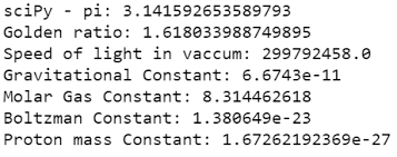
SciPy has a large number of constants, which are used to show different magnitudes. Among these we have:

Metrics

As their name indicates, these constants will be used to represent distances, and they will always show us their value in meters. Following scientific notation, these will have values ranging from zeptometers (Equivalent to 10 to the -21 meters or one sextillionth of a meter) to yottameters (10 to the -24).

from scipy import constants

print(constants.yotta)
print(constants.kilo)
print(constants.zepto)

>>>
1e+24
1000.0
1e-21

Binary

As we know, when working with memories, we will always talk about bits and bytes. In this case, each constant will be represented taking bytes as a unit. These can range from kibibytes (The specific term to describe 1024 bytes, for which we usually use the more informal 'kilobyte') to yobibytes, which is equivalent to 1208925819614629174706176 bytes.

from scipy import constants

print(constants.kibi)
print(constants.mebi) # mebibytes or megabytes
print(constants.yobi)

>>>
1024
1048576
1208925819614629174706176

Mass

Mass is expressed with the unit of kilograms, which will convert from any constant, whether pounds, tons, ounces or carats:

from scipy import constants

print(constants.gram)
print(constants.metric_ton) #1000.0
print(constants.lb) # You can also write constants.pound / You can also write constants.pound
print(constants.oz) # Also ounce / Also ounce
print(constants.carat)

>>>
0.001
1000.0
0.45359236999999997
0.028349523124999998
0.0002

In addition to these three, we have many more constants, ranging from power and speed to force and energy, to see all the constants you can use, you just have to write:

print(dir(constants))

>>>
['Avogadro', 'Boltzmann', 'Btu', 'Btu_IT', 'Btu_th', 'ConstantWarning', 'G', 'Julian_year', 'N_A', 'Planck', 'R', 'Rydberg', 'Stefan_Boltzmann', 'Wien', '__all__', '__builtins__', '__cached__', '__doc__', '__file__', '__loader__', '__name__', '__package__', '__path__', '__spec__', '_codata', '_constants', '_obsolete_constants', 'acre', 'alpha', 'angstrom', 'arcmin', 'arcminute', 'arcsec', 'arcsecond', 'astronomical_unit', 'atm', 'atmosphere', 'atomic_mass', 'atto', 'au', 'bar', 'barrel', 'bbl', 'blob', 'c', 'calorie', 'calorie_IT', 'calorie_th', 'carat', 'centi', 'codata', 'constants', 'convert_temperature', 'day', 'deci', 'degree', 'degree_Fahrenheit', 'deka', 'dyn', 'dyne', 'e', 'eV', 'electron_mass', 'electron_volt', 'elementary_charge', 'epsilon_0', 'erg', 'exa', 'exbi', 'femto', 'fermi', 'find', 'fine_structure', 'fluid_ounce', 'fluid_ounce_US', 'fluid_ounce_imp', 'foot', 'g', 'gallon', 'gallon_US', 'gallon_imp', 'gas_constant', 'gibi', 'giga', 'golden', 'golden_ratio', 'grain', 'gram', 'gravitational_constant', 'h', 'hbar', 'hectare', 'hecto', 'horsepower', 'hour', 'hp', 'inch', 'k', 'kgf', 'kibi', 'kilo', 'kilogram_force', 'kmh', 'knot', 'lambda2nu', 'lb', 'lbf', 'light_year', 'liter', 'litre', 'long_ton', 'm_e', 'm_n', 'm_p', 'm_u', 'mach', 'mebi', 'mega', 'metric_ton', 'micro', 'micron', 'mil', 'mile', 'milli', 'minute', 'mmHg', 'mph', 'mu_0', 'nano', 'nautical_mile', 'neutron_mass', 'nu2lambda', 'ounce', 'oz', 'parsec', 'pebi', 'peta', 'physical_constants', 'pi', 'pico', 'point', 'pound', 'pound_force', 'precision', 'proton_mass', 'psi', 'pt', 'short_ton', 'sigma', 'slinch', 'slug', 'speed_of_light', 'speed_of_sound', 'stone', 'survey_foot', 'survey_mile', 'tebi', 'tera', 'test', 'ton_TNT', 'torr', 'troy_ounce', 'troy_pound', 'u', 'unit', 'value', 'week', 'yard', 'year', 'yobi', 'yocto', 'yotta', 'zebi', 'zepto', 'zero_Celsius', 'zetta']

Optimizers

Shoutout to Python Guides

Optimizers are a series of procedures that allow us to perform various operations such as finding the roots of a given equation or finding the minimum maximums of a function.

If you don't have a very clear notion of what the roots or maximums and minimums are, don't worry, we will give a brief explanation of each one.

Roots

If we have an equation that is graphed on the coordinate axis:

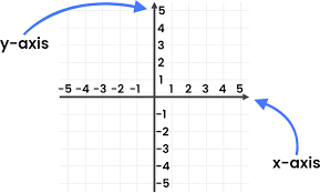
Shoutout to House of Math

So, we know that the roots are those points where the curve of a function passes through point 0 of the y-axis. If we take for example the following function:

y = 2x - 5

We know that when searching for roots, the value of the y-axis will be zero according to the definition. Thus, we would have the following:

0 = 2x - 5

And to find the root, we will only have to solve for x. Thus:

2x = 5
x = 5/2 or 2.5

So we know that the root has a value of 2.5, which will be the point where the drawn line will cross the value of y = 0. However, in order to have a more accurate graph, we must take other points.

If we want to do this in a simple way, we first identify the independent term in the equation (The one that does not have x) which in this case is - 5, which will be the point where the line crosses the value of 0 on the because if x is 0, the 2 cancels out and remains - 5).

Furthermore, for more precision, a good practice is to consider the number that accompanies the x as a fraction, where we would have 2/1, which represents that every time the function moves two positions on the y axis, it will move a position on the x axis. Thus, if we finally graph, we will have the following:

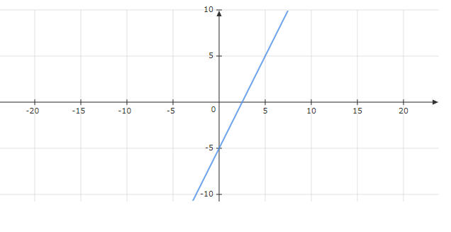
With which the root is fulfilled. However, as the degree of complexity of a function increases, so does the way its roots are analytically determined. This is why we use computerized algorithms, in this case Scipy, to determine the root. If, for example, we have the function x-cos(x):

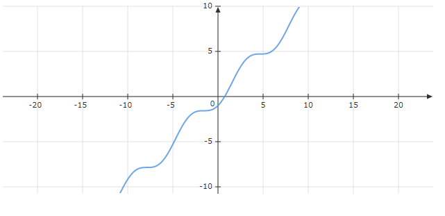
Then it becomes more difficult for us to determine the value of the root quickly. For this we simply use the Scipy optimizer module and import the root function into it. To carry out this operation we must determine a function in the following way:

from scipy.optimizer import root
from math import cos

def eqn(x):
return x - cos(x)

Note: Remember that to use trigonometric functions in Python we must import the math module.

And now to return the root of the function, we create a variable and use root, taking as parameters:

• The name of the function (In this case eqn).
• An initial prediction of what we think the value of the root is (Don't be afraid of being wrong, if you don't enter the correct value the root will give it to you anyway).

And thus, the information about the root will be stored in the x attribute of the root class object. So, to see the root:

from scipy.optimizer import root
from math import cos

def eqn(x):
return x - cos(x)

myroot = root(eqn, 1)

print(myroot.x)

>>> [0.73908513]

Which is the root of our function.

Note: There are functions with more than one root. If you want to find them, you can use the same procedure with root without any problem.

Minimums

By having a curve of the following shape:

f(x) = y = x^2 + 6x + 8

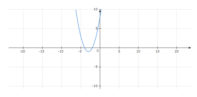
We have that this function reaches a lower point which it cannot exceed, as can be seen in the extreme that it reaches the asymptote before rising again. This is what is known as a minimum.

Now, in other functions the opposite happens. There is a maximum point which cannot be exceeded, this being the maximum.

However, a distinction can be made between two types of maximums/minima, which are:

• The absolute minimum/maximum, which is the point that cannot be exceeded in the entire function and below/above which there are no values for the function.
• Local minimums/maximums are those that take a certain interval (For example, all values from -2 to 2) and identify which is the highest value of this point.

Now if we take our previous function. The first thing we must do is look for a derivative. Because?

You see, one of the definitions for the derivative is the slope or inclination of a tangent line to the function (That is, a line that grazes or touches the graph of the function, but does not cut it). For example:

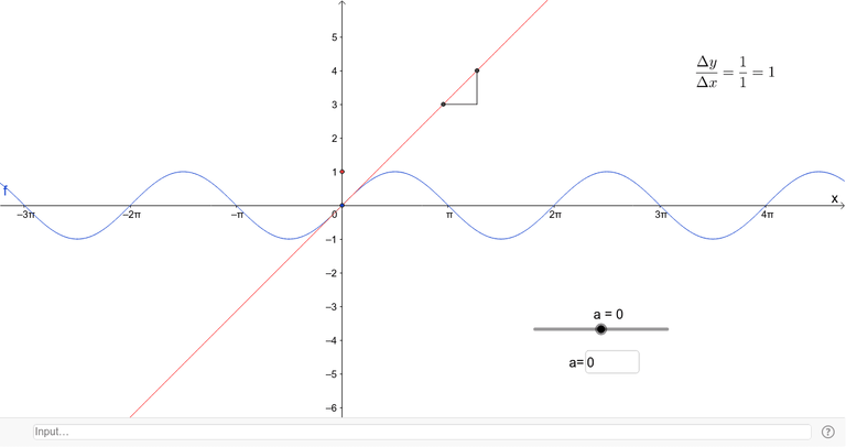
Shoutout to GeoGebra

For this sinusoidal function, the derivative would allow us to calculate the inclination of the red line, which as we see touches the function but does not touch it.

So what does this have to do with highs and lows? A lot.

If we want to find the inclination of a slope line at the maximum and minimum point of a function, we know that the inclination will be 0, so a fairly simple way to find the maximum and minimum of a function is simply by looking for all the values where the derivative of our function is 0.

For example, taking again f(x) = x^2 + 6x + 8, if we differentiate, we will have:

f(x)' = 2x + 6

Note: Let me know if you want an article on derivatives :)

Now, we have to find the values of x that make f(x)' be 0. If we see the numbers that accompany it (2 multiplying and 6 adding), we know that the value will be -3:

f(x)' = 2 * (-3) + 6 = -6 + 6 = 0

Here, we know that the only local minimum that the function has will be x = -3. Furthermore, there is no maximum, since when observing the function, we see that it continues to infinity as it continues to increase to the right.

Although this is one of the methods that can be used, there are others that will lead us to the same result. However, this is a good start.

Now, if we wanted to do the same thing through scipy, we would have to use another function from the optimize module, called minimize.

To use minimize, we have to use the following parameters:

• The name of the function for which the minimum is being searched.
• A prediction of the value of the minimum.
• The method to use.

In addition to the callback parameters, which will be a function to execute after each optimization operation, as well as a dictionary with disp parameters, to print a verbose entry and gtol to enter error tolerance.

So, if we wanted to find the minimum, we just define our function and apply minimize on a new variable:

from scipy.optimize import minimize

def eqn(x):
   return x**2 + 6*x + 8

min_function = minimize(eqn, -1, method='BFGS')

print(mymin)

>>>
fun: -1.0
  hess_inv: array([[0.5]])
       jac: array([0.])
   message: 'Optimization terminated successfully.'
      nfev: 9
       nit: 2
      njev: 3
    status: 0
   success: True
         x: array([-3.00000002])

Thus, we can see detailed information about the function, including the minimum, displayed in the array.

We can see that Scipy is a tool with great potential when working in Data Science. However, its capabilities do not stop only at these functions, since we can perform countless operations with them, which make it a favorite among its users.

I hope that with this article you have been able to understand how SciPy works, its constants and how to search for roots as well as minima. In this way, we are only getting started. If you want to learn more about Data Science. Keep reading.

See you!

Thank you for your support and good luck!

Un paso en Data Science

Shoutout to Real Python

En este artículo encontrarás:

• Introducción
• ¿Qué es SciPy?
• Usando SciPy
• Constantes con SciPy
• Optimizadores

¡Bienvenido de nuevo a Coding Basics!

Sé que esta semana ha sido floja respecto a la publicación de nuevas ediciones. Sin embargo, no pienso dejar de publicar.

En los artículos previos aprendimos todo lo necesario para empezar a manejar la información de archivos csv en Pandas y realizar distintas operaciones estadísticas así como usar estos datos para graficar por medio de matplotlib.

Sin embargo, pandas por si solo no será suficiente para aprovechar al maximo esta librería. Es por esto, que surgen gran cantidades de paquetes los cuales nos permiten trabajar en campos más amplios como son el Data Science y el Machine Learning.

Entre estas, se encuentra una librería muy popular, que al trabajar con Pandas nos permitirá obtener información realmente interesante, llamada SciPy.

Si quieres saber como manejar operaciones matemáticas complejas por medio del uso de una librería, solo sigue leyendo.

¡Comencemos!

¿Qué es SciPy?

Shoutout to LA-CoNGA physics

SciPy es una biblioteca de código abierto para Python, con operaciones que se encargan de realizar operaciones de computación científica, es decir, resolver problemas matemáticos complejos por medio de algoritmos o programas de computadora.

Recordamos que en ediciones anteriores hablamos sobre una librería que nos permitía responder operaciones matemáticas: NumPy. Pues bien, SciPy está basado en la colección de datos de NumPy, creada por Travis Oliphant, quien también es uno de los creadores de SciPy.

Entre algunos de los módulos que se encuentra dentro de la biblioteca SciPy podemos ver algunos dedicados al algebra lineal, el procesamiento de señales, las derivadas e incluso las integraciones.

Así pues, ya sabemos que es Scipy. Sin embargo, ¿Cómo podemos usar SciPy?

Usando SciPy

Shoutout to Wikipedia

El primer paso para usar SciPy es cerciorarnos de que esté instalado. Para esto, nos dirigimos a nuestra línea de comandos (CMD, Powershell, o Unix) y aquí, teniendo pip instalado (Si no sabes como instalarlo, puedes ver este artículo), escribimos:

pip install scipy

Una vez que veamos que tenemos scipy instalado, podremos dirigirnos a nuestro IDE e importar alguno de sus módulos, como puede ser el llamado constants, de la siguiente manera:

from scipy import constants

Y de aquí, solo queda usar sus métodos y funciones de acuerdo a la documentación de cada módulo:

from scipy import constants 

print(constants.pi)

>>> 3.141592653589793

Constantes con SciPy

Shoutout to GeeksforGeeks

Si verificamos nuesrta definición de constante:

Una constante es una variable la cual tiene un valor asignado, fijo e inmutable.

Es decir, si tomamos el valor de pi, que es 3.141592653, sabemos que este valor nunca cambiará, haciendo que esta sea una constante.

SciPy dispone de una gran cantidad de constantes, las cuales son usadas para mostrar distintas magnitudes. Entre estas tenemos:

Métricas

Como su nombre lo indica, estas constantes se usarán para representar distancias, y siempre nos mostrarán su valor en metros. Siguiendo la notación científica, estos tendrán valores que van desde los zeptómetros (Equivalente a 10 a la -21 metros o una sextillonésima de metro) hasta los yottámetros (10 a la -24).

from scipy import constants

print(constants.yotta)
print(constants.kilo)
print(constants.zepto)

>>>
1e+24
1000.0
1e-21

Binarias

Como sabemos, al trabajar con memorias, hablaremos siempre de bits y bytes. En este caso, cada constante será representada tomando bytes como unidad. Estas pueden ir desde los kibibytes (El término específico para describir 1024 bytes, para el que solemos usar el más informal 'kilobyte') hasta los yobibytes, que equivale a 1208925819614629174706176 bytes.

from scipy import constants

print(constants.kibi)
print(constants.mebi) # mebibytes or megabytes
print(constants.yobi)

>>>
1024
1048576
1208925819614629174706176

Masa

La masa se expresa con la unidad de kilogramos, la cual hará la conversión desde cualquier constante, ya sean libras, toneladas, onzas o quilates:

from scipy import constants

print(constants.gram)
print(constants.metric_ton)  #1000.0
print(constants.lb) # You can also write constants.pound / También puedes escribir constants.pound
print(constants.oz) # Also ounce / También ounce
print(constants.carat)

>>>
0.001
1000.0
0.45359236999999997
0.028349523124999998
0.0002

Además de estas tres, tenemos muchas más constantes, que van desde la potencia, y la velocidad hasta la fuerza y la energía, para ver todas las constantes que puedes usar, solo debes escribir:

print(dir(constants))

>>>
['Avogadro', 'Boltzmann', 'Btu', 'Btu_IT', 'Btu_th', 'ConstantWarning', 'G', 'Julian_year', 'N_A', 'Planck', 'R', 'Rydberg', 'Stefan_Boltzmann', 'Wien', '__all__', '__builtins__', '__cached__', '__doc__', '__file__', '__loader__', '__name__', '__package__', '__path__', '__spec__', '_codata', '_constants', '_obsolete_constants', 'acre', 'alpha', 'angstrom', 'arcmin', 'arcminute', 'arcsec', 'arcsecond', 'astronomical_unit', 'atm', 'atmosphere', 'atomic_mass', 'atto', 'au', 'bar', 'barrel', 'bbl', 'blob', 'c', 'calorie', 'calorie_IT', 'calorie_th', 'carat', 'centi', 'codata', 'constants', 'convert_temperature', 'day', 'deci', 'degree', 'degree_Fahrenheit', 'deka', 'dyn', 'dyne', 'e', 'eV', 'electron_mass', 'electron_volt', 'elementary_charge', 'epsilon_0', 'erg', 'exa', 'exbi', 'femto', 'fermi', 'find', 'fine_structure', 'fluid_ounce', 'fluid_ounce_US', 'fluid_ounce_imp', 'foot', 'g', 'gallon', 'gallon_US', 'gallon_imp', 'gas_constant', 'gibi', 'giga', 'golden', 'golden_ratio', 'grain', 'gram', 'gravitational_constant', 'h', 'hbar', 'hectare', 'hecto', 'horsepower', 'hour', 'hp', 'inch', 'k', 'kgf', 'kibi', 'kilo', 'kilogram_force', 'kmh', 'knot', 'lambda2nu', 'lb', 'lbf', 'light_year', 'liter', 'litre', 'long_ton', 'm_e', 'm_n', 'm_p', 'm_u', 'mach', 'mebi', 'mega', 'metric_ton', 'micro', 'micron', 'mil', 'mile', 'milli', 'minute', 'mmHg', 'mph', 'mu_0', 'nano', 'nautical_mile', 'neutron_mass', 'nu2lambda', 'ounce', 'oz', 'parsec', 'pebi', 'peta', 'physical_constants', 'pi', 'pico', 'point', 'pound', 'pound_force', 'precision', 'proton_mass', 'psi', 'pt', 'short_ton', 'sigma', 'slinch', 'slug', 'speed_of_light', 'speed_of_sound', 'stone', 'survey_foot', 'survey_mile', 'tebi', 'tera', 'test', 'ton_TNT', 'torr', 'troy_ounce', 'troy_pound', 'u', 'unit', 'value', 'week', 'yard', 'year', 'yobi', 'yocto', 'yotta', 'zebi', 'zepto', 'zero_Celsius', 'zetta']

Optimizadores

Shoutout to Python Guides

Los optimizadores son una serie de procedimientos que nos permiten realizar varias operaciones como lo son encontrar las raíces de una ecuación determinada o buscar los mínimos máximos de una función.

Si no tienes una noción muy clara de lo que son las raíces o máximos y mínimos, no te preocupes, le daremos una breve explicación a cada una.

Raíces

Si tenemos una ecuación que se grafica en el eje de las coordenadas:

Shoutout to House of Math

Entonces, sabemos que las raíces son aquellos puntos donde la curva de una función pase por el punto 0 del eje y. Si tomamos por ejemplo la siguiente función:

y = 2x - 5

Sabemos que al buscar las raíces, el valor del eje y será cero según la definición. Así, tendríamos lo siguiente:

0 = 2x - 5

Y para encontrar la raíz, solo tendremos que despejar a x. De esta forma:

2x = 5
x = 5/2 o 2.5

Con lo que sabemos que la raíz tiene un valor de 2,5, que será el punto donde la recta trazada tomará cruzará el valor de y = 0. Sin embargo, en orden de tener una gráfica más precisa, debemos de tomar otros puntos.

Si queremos hacer esto de forma sencilla, primero identificamos el término independiente en la ecuación (El que no tiene x) que en este caso es - 5, lo cual será el punto en que la recta cruce el valor de 0 del eje x (Debido a que si x es 0, el 2 se cancela y queda - 5).

Además, para más precisión, una buena práctica es considerar el número que acompaña a la x como una fracción, donde tendríamos a 2/1, lo cual que representa que cada vez que la función se mueve dos posiciones en el eje y, se moverá una posición en el eje x. Así, si graficamos finalmente, tendremos lo siguiente:

Con lo que se cumple la raíz. Sin embargo, al aumentar el grado de complejidad de una función, también lo hace la forma de determinar de manera analítica sus raíces. Es por esto, que hacemos uso de algoritmos computarizados, en este caso a Scipy, para determinar la raíz. Si por ejemplo, tenemos la función x-cos(x):

Entonces se nos hace más complicado determinar el valor de la raíz rápidamente. Para esto simplemente hacemos uso del módulo de Scipy optimizer y le importamos la función root. Para llevar a cabo esta operación debemos de determinar una función de la siguiente manera:

from scipy.optimizer import root
from math import cos

def eqn(x):
    return x - cos(x)

Nota: Recordar que para usar funciones trigonométricas en Python debemos de importar el módulo math.

Y ahora para retornar la raíz de la función, creamos una variable y usamos root, tomando como parámetros:

• El nombre de la función (En este caso eqn).
• Una predicción inicial de lo que pensemos que sea el valor de la raíz (No tengas miedo de equivocarte, si no colocas el valor correcto el root te lo dará igualmente).

Y así, la información sobre la raíz quedará guardada en el atributo x del objeto de la clase root. Así, para ver la raíz:

from scipy.optimizer import root
from math import cos

def eqn(x):
    return x - cos(x)

myroot = root(eqn, 1)

print(myroot.x)

>>> [0.73908513]

Lo cual es la raíz de nuestra función.

Nota: Existen funciones con más de una raíz. Si las quieres encontrar, puedes usar el mismo procedimiento con root sin ningún problema.

Mínimos

Al tener una curva de la siguiente forma:

f(x) = y = x^2 + 6x + 8

Tenemos que esta función alcanza un punto más bajo el cual no puede superar, como se puede ver en el extremo que alcanza la asíntota antes de volver a ascender. Esto es lo que se conoce como mínimo.

Ahora bien, en otras funciones pasa la contrario. Existe un punto máximo el cual no se puede superar, siendo este el máximo.

Sin embargo, se puede hacer una distinción entre dos tipos de máximos/mínimos, los cuales son:

• Los mínimos/máximos absolutos, que son el punto que no se puede superar en toda la función y debajo/encima del cual no existen valores para la función.
• Los mínimos/máximos locales, son aquellos que toman un intervalo determinado (Por ejemplo, todos los valores de -2 a 2) e identifica cual es el valor más de este punto.

Ahora bien, si tomamos nuestra función anterior. Lo primero que debemos de hacer es buscar una derivada. ¿Por qué?

Verás, una de las definiciones para la derivada es la pendiente o inclinación de una recta tangente en la función (Es decir, una recta que roza o toca la gráfica de la función, pero no la corta). Por ejemplo:

Shoutout to GeoGebra

Para esta función senoidal, la derivada nos permitiría calcular la inclinación de la recta roja, que como vemos toca la función más no la toca.

Entonces, ¿Qué tiene que ver esto con los máximos y los mínimos? Mucho.

Si queremos buscar la inclinación una recta pendiente en el punto máximo y mínimo de una función, sabemos que la inclinación será 0, por lo que una forma bastante sencilla de encontrar los máximos y los mínimos de una función es simplemente buscando todos los valores donde la derivada de nuestra función sea 0.

Por ejemplo, tomando de nuevo a f(x) = x^2 + 6x + 8, si derivamos, tendremos:

f(x)' = 2x + 6

Nota: Hazme saber si quiere un artículo sobre las derivadas :)

Ahora, tenemos que buscar los valores de x que hagan que f(x)' sea 0. Si vemos los números que la acompañan (2 multiplicando y 6 sumando), sabemos que el valor será -3:

f(x)' = 2 * (-3) + 6 = -6 + 6 = 0

Aquí, sabemos que el único mínimo local que tiene la función será x = -3. Además, no existe máximo, ya que al observa la función, vemos que esta continua al infinito a medida que se sigue incrementando a la derecha.

Si bien este es uno de los métodos que se puede usar, existen otros qu nos llevarán al mismo resultado. Sin embargo, este es un buen comienzo.

Ahora bien, si quisieramos hacer lo mismo por medio de scipy, tendríamos que usar otra función del módulo optimize, llamada minimize.

Para usar minimize, tenemos que usar los siguientes parámetros:

• El nombre de la función a la que se le está buscando el mínimo.
• Una predicción del valor del mínimo.
• El método a utilizar.

Además de los parámetros de callback, que será una función a ejecutar después de cada operación de optimización, así como un diccionario con parámetros de disp, para imprimir una inscripción detallada y gtol para introducir la tolerancia de error.

Así, si quisieramos buscar el mínimo, solo definimos nuestra función y aplicamos minimize en una nueva variable:

from scipy.optimize import minimize

def eqn(x):
  return x**2 + 6*x + 8

min_function = minimize(eqn, -1, method='BFGS')

print(mymin)

>>> 
fun: -1.0
 hess_inv: array([[0.5]])
      jac: array([0.])
  message: 'Optimization terminated successfully.'
     nfev: 9
      nit: 2
     njev: 3
   status: 0
  success: True
        x: array([-3.00000002])

Así, podemos ver información detallada sobre la función, incluyendo el mínimo, que se muestra en el arreglo.

Podemos ver que Scipy es una herramienta con un gran potencial a la hora de trabajar en Data Science. Sin embargo, sus capacidades no se quedan solo en estas funciones, ya que podemos realizar infinidad de operaciones con estas, los cuales la hacen un favorito entre sus usuarios.

Espero que con este artículo hayas podido entender como funciona SciPy, sus constantes y como buscar raíces así como mínimos. De esta forma, solo estamos empezando. Si quieres aprender más sobre Data Science. Sigue leyendo.

¡Nos vemos!

¡Gracias por tu apoyo y buena suerte!