Active filters: Graphical analysis EN/ES

Studying the different types of active filters might require advanced knowledge in electronic engineering and calculus since differential equations are required to evaluate some answers and circuit knowledge to implement the correct designs.

I do not intend to create complex topics because I understand that I write for a global audience and my intention in creating this blog has always been to present electronics in the easiest way to understand without affecting the quality of our designs.

With the technologies we have today differential equations and complex calculations can be omitted because there are design applications that take care of it, however it is necessary to know the parameters and principles of operation to understand and correctly apply the design technologies.

That is where my focus is in this series of articles, that the reader can become familiar with filters at the surface level and be able to design them using applications that take care of the complex calculations. So today we are going to see what approximations are and in the act we will learn how to interpret the graphs.

---

Estudiar los distintos tipos de filtros activos podría requerir conocimientos avanzados en ingeniería electrónica y cálculo ya que se requiere de ecuaciones diferenciales para evaluar algunas respuestas y conocimientos de circuitos para implementar los diseños correctos.

No pretendo crear temas complejos porque entiendo que escribo para un público global y mi intención al crear este blog siempre ha sido presentar la electrónica de la forma más fácil de comprender sin afectar la calidad de nuestros diseños.

Con las tecnologías que disponemos actualmente las ecuaciones diferenciales y los cálculos complejos pueden omitirse porque existen aplicaciones de diseño que se encargan de ello, sin embargo es necesario conocer los parametros y principios de funcionamiento para poder comprender y aplicar de forma correcta las tecnologías de diseño.

Es ahí donde está centrado mi enfoque en esta serie de artículos, que el lector se pueda familiarizar con los filtros a nivel superficial y pueda ser capaces de diseñarlos mediante aplicaciones que se encarguen de los cálculos complejos. Así que hoy vamos a ver que son las aproximaciones y en el acto aprenderemos a interpretar las gráficas.

---

Graphical analysis

We can rely on several graphs to analyze our designs, the way a graph is constructed is simple, a y-axis as a function of an x-axis, the only thing that will change will be the variables that we want to represent on each axis.

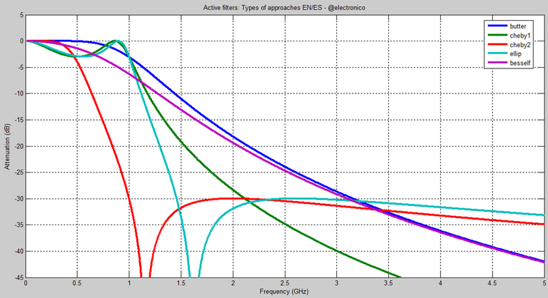
We could represent for example the phase shift with respect to frequency, the output magnitude with respect to frequency, attenuation with respect to frequency. If you notice everything is with respect to the frequency because it is the fundamental variable that we use to design our filters and the work of a filter is precisely to vary its behavior with respect to the change of frequencies.

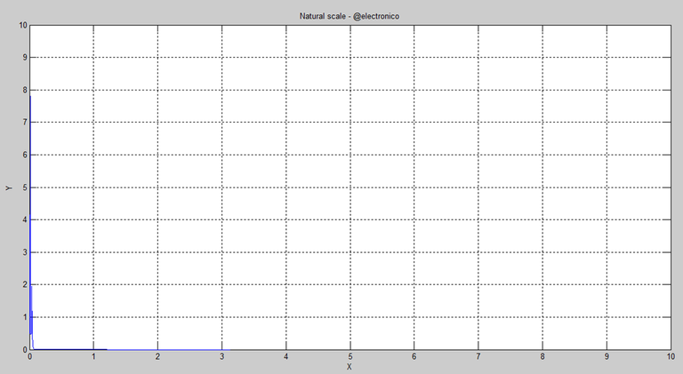
On the other hand we have the scales, in our case we will consider two types: natural when the distances between each representative point is the same, if my first point is 1 the second will be 2 the third 3 and so on and each frame of a grid will have the same value.

---

Podemos apoyarnos en varias gráficas para analizar nuestros diseños, la forma como se construye una gráfica es sencilla, un eje y en función de un eje x, lo unico que cambiara sera las variables que deseamos representar en cada eje.

Podríamos representar por ejemplo el cambio de fase respecto a la frecuencia, la magnitud de salida respecto a la frecuencia, atenuación respecto a la frecuencia. Si lo notas todo está respecto a la frecuencia porque es la variable fundamental que usamos para diseñar nuestros filtros y el trabajo de un filtro es precisamente variar su comportamiento respecto al cambio de frecuencias.

Por otro lado tenemos las escalas, en nuestro caso consideraremos dos tipos: natural cuando las distancias entre cada punto representativo es la misma, si mi primer punto es el 1 el segundo sera el 2 el tercero el 3 y así en lo sucesivo y cada cuadro de un grid tendrá el mismo valor.

---

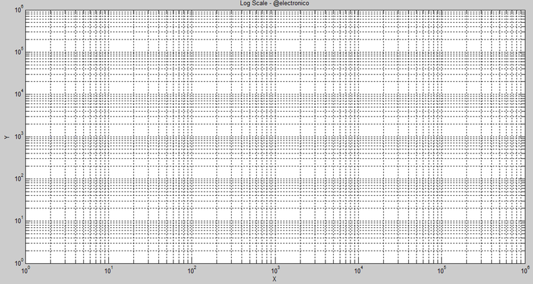
When a very large range of values needs to be represented, the logarithmic scale is used, it is based on a logarithm of base 10 where the next reference point will be ten times greater than the previous one.

---

Cuando se necesita representar un rango muy grande de valores se utiliza la escala logarítmica, está basada en un logaritmo de base 10 donde el siguiente punto de referencia sera diez veces mayor al anterior.

---

Now that we have the graphic sheet to represent our data we must choose who will be on the Y axis and who will be on the X axis, the variables that we place there will help us to analyze the behavior of our designs, the X axis in most cases is represented by the frequency in Hz or rad/sec but almost always will be the frequency variable there.

In the Y variable we will place the variable that we want to analyze since we will be able to appreciate which is its behavior in front of the different values of frequency. Since we are designing a filter the first thing we want to know is its ability to block signals at unwanted frequencies. The efficiency of the filter will depend on that, then we can analyze other things such as phase shift, output magnitude.

Attenuation refers to how much signal is lost or removed. For a constant input voltage the attenuation can be calculated as the output value at any frequency divided by the output value for medium frequencies.

---

Ahora que tenemos la hoja gráfica para representar nuestros datos debemos escoger quien estará en el eje de las Y y quien en el de la X, las variables que coloquemos ahí nos ayudarán a analizar el comportamiento de nuestros diseños, el eje de las X en la mayor parte de los casos está representado por la frecuencia en Hz o rad/seg pero casi siempre sera la variable frecuencia ahí.

En la variable de las Y colocaremos la variable que deseamos analizar ya que podremos apreciar cuál es su comportamiento frente a los distintos valores de frecuencia. Ya que estamos diseñando un filtro lo primero que queremos saber es su capacidad de bloquear las señales a frecuencias no deseadas. De eso dependerá la eficiencia del mismo, luego podremos analizar otras cosas como el cambio de fase, magnitud de salida.

La atenuación se refiere a cuanta señal se pierde o se elimina. Para un voltaje de entrada constante la atenuación se puede calcular como el valor de salida en cualquier frecuencia dividido entre el valor de la salida para frecuencias medias.

---

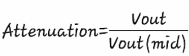
Generally the attenuation is expressed in decibels, if we have the voltage output values at the frequency we want to calculate the attenuation and the voltage output values at medium frequencies we can use the following formula to calculate the attenuation in decibels.

---

Generalmente la atenuación se expresa en decibelios, si tenemos los valores de salida de voltaje a la frecuencia que queremos calcular la atenuación y los valores de salida de voltaje a frecuencias medias podemos usar la siguiente fórmula para calcular la atenuación en decibelios.

---

For example, an attenuation of 3 dB means that the output voltage is 0.707 of its value in the mid frequencies, if 6 dB the output is 0.5 of its value in the mid frequencies, if 12 dB, that the output voltage is 0.25 of its value in the mid frequencies and we can calculate any value to know how effective our filter is.

Attenuation is not desired in the passband but a loss of 0.5dB is usually sacrificed to obtain a better attenuation of the removed band.

---

Por ejemplo, una atenuación de 3 dB significa que la tensión de salida es 0,707 de su valor en las frecuencias medias, si 6 dB la salida es 0,5 de su valor en las frecuencias medias, si 12 dB, que la tensión de salida es 0,25 de su valor en las frecuencias medias y podemos así calcular cualquier valor para conocer qué tan efectivo es nuestro filtro.

La atenuación no es deseada en la banda pasante pero se suele sacrificar una pérdida de 0.5dB para obtener una mejor atenuación de la banda eliminada.

---

Butterworth Approximation

When we refer to approximations it does not mean that each type of approximation needs a schematic modification in the circuit, often it is enough to change some values in the components to obtain the responses that comply with the approximation without the need to add, remove or move components between one filter or another.

In the Butterworth approximation the attenuation in most of the passband is zero (no power is sacrificed from the area where the frequency is acceptable to the filter) and gradually decreases after the cutoff frequency.

The attenuation slope for this approach can be calculated with the following formula:

---

Cuando nos referimos a las aproximaciones no quiere decir que cada tipo de aproximación necesite una modificación esquemática en el circuito, a menudo solo basta con cambiar algunos valores en los componentes para obtener las respuestas que cumplan con la aproximación sin que sea necesario añadir, quitar o mover componentes entre un filtro u otro.

En la aproximación de Butterworth la atenuación en la mayor parte de la banda pasante es cero (no se sacrifica potencia de la zona en la que la frecuencia es aceptable para el filtro) y disminuye gradualmente luego de la frecuencia de corte.

La pendiente de atenuación para esta aproximación se puede calcular con la siguiente fórmula:

---

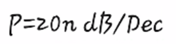
Where P is the attenuation slope and n the order of the filter, we can use MatLab to illustrate the behavior of a Butterworth filter as we increase the order, we will do it 2 by 2 up to order 10. To do this we will use the following code:

---

Donde P es la pendiente de atenuación y n el orden del filtro, podemos usar MatLab para ilustrar el comportamiento de un filtro Butterworth a medida que aumentamos el orden, lo haremos de 2 en 2 hasta el orden 10. Para ello utilizaremos el siguiente código:

---

clear all

clc

n=2;

wn=0.7;

for n=2:2:10

[num den]=butter(n,wn,'Low');

ft=tf(num,den)

[h w]=freqz(num,den);

plot(w,abs(h), 'LineWidth',2)

title('Butterworth - @electronico')

xlabel('(Hz)')

ylabel('dB')

grid on

pause(2)

hold on

end

And this generates the following result:

---

Y esto nos genera el siguiente resultado:

---

We can notice how the slope increases as the filter order increases.

There are still other approaches to study but I don't want to saturate you with content, so for now we end this article up to here 😉.

See you in the comments section 👍.

---

Podemos notar como la pendiente aumenta a medida que aumenta el orden del filtro.

Aún faltan estudiar otras aproximaciones pero no quiero saturarlos de contenido, así que por ahora terminamos este artículo hasta aquí. 😉.

Nos vemos en las sección de comentarios 👍.

---

---

---

---

---

---

---

---

https://images.ecency.com/p/3W72119s5BjW4PvRk9nXBzqrPWMsMTjNrXDPFFf12CAfRz5MY8jCm5vGDUj7o96hwAT3YCMBJgcTgcWmsqeuBbZL1YbmxtaV4gyfByenDkmAkgv6rkm9ZP.webp?format=webp&mode=fit